Entropy (thermodynamics)

From Knowino

Jump to: navigation, search

Entropy is a function of the state of a thermodynamic system. It is a size-extensive^[1] quantity, invariably denoted by S, with dimension energy divided by absolute temperature (SI unit: joule/K). Entropy has no analogous mechanical meaning—unlike volume, a similar size-extensive state parameter. Moreover entropy cannot be measured directly, there is no such thing as an entropy meter, whereas state parameters like volume and temperature are easily determined. Consequently entropy is one of the least understood concepts in physics.^[2]

Excerpt from Clausius (1865)^[3].
Translation: Searching for a descriptive name for S, one could — like it is said of the quantity U that it is the heat and work content of the body — say of the quantity S that it is the transformation content of the body. As I deem it better to derive the names of such quantities — that are so important for science — from the antique languages, so that they can be used without modification in all modern languages, I propose to call the quantity S the entropy of the body, after the Greek word for transformation, ἡ τροπή. I have deliberately constructed the word entropy to resemble as much as possible the word energy, since both quantities to be named by these words are so closely related in their physical meaning that a certain similarity in their names seems appropriate to me.

The state variable "entropy" was introduced by Rudolf Clausius in 1865,^[3] see the inset for his text, when he gave a mathematical formulation of the second law of thermodynamics.

The traditional way of introducing entropy is by means of a Carnot engine, an abstract engine conceived of by Sadi Carnot in 1824^[4] as an idealization of a steam engine. Carnot's work foreshadowed the second law of thermodynamics. The "engineering" manner—by an engine—of introducing entropy will be discussed below. In this approach, entropy is the amount of heat (per degree kelvin) gained or lost by a thermodynamic system that makes a transition from one state to another. The second law states that the entropy of an isolated system increases in spontaneous (natural) processes leading from one state to another, whereas the first law states that the internal energy of the system is conserved.

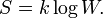
In 1877 Ludwig Boltzmann^[5] gave a definition of entropy in the context of the kinetic gas theory, a branch of physics that developed into statistical thermodynamics. Boltzmann's definition of entropy was furthered by John von Neumann^[6] to a quantum statistical definition. The quantum statistical point of view, too, will be reviewed in the present article. In the statistical approach the entropy of an isolated (constant energy) system is k_B logΩ, where k_B is Boltzmann's constant and the function log stands for the natural (base e) logarithm. Ω is the number of different wave functions ("microstates") of the system belonging to the system's "macrostate" (thermodynamic state). The number Ω is the multiplicity of the macrostate; for an isolated system, where the macrostate is of definite energy, Ω is its degeneracy. For a system of about 10²³ particles, Ω is on the order of 10^10²³, that is the entropy is on the order of 10²³×k_B ≈ R, the molar gas constant.

Not satisfied with the engineering type of argument, the mathematician Constantin Carathéodory gave in 1909 a new axiomatic formulation of entropy and the second law of thermodynamics.^[7] His theory was based on Pfaffian differential equations. His axiom replaced the earlier Kelvin-Planck and the equivalent Clausius formulation of the second law and did not need Carnot engines. Carathéodory's work was taken up by Max Born,^[8] and it is treated in a few monographs.^[9]^[10] ^[11] Since it requires more mathematical knowledge than the traditional approach based on Carnot engines, and since this mathematical knowledge is not needed by most students of thermodynamics, the traditional approach, which depends on some ingenious thought experiments, is still dominant in the majority of introductory works on thermodynamics.

[edit] Specific entropy

Entropy (as the extensive property mentioned above) has corresponding intensive (size-independent) properties for pure materials. A corresponding intensive property is specific entropy, which is entropy per mass of substance involved. Specific entropy is denoted by a lower case s, with dimension of energy per absolute temperature and mass [SI unit: joule/(K·kg)]. If a molecular mass or number of moles involved can be assigned, then another corresponding intensive property is molar entropy, which is entropy per mole of the compound involved, or alternatively specific entropy times molecular mass. There is no universally agreed upon symbol for molar properties, and molar entropy has been at times confusingly symbolized by S, as in extensive entropy. The dimensions of molar entropy are energy per absolute temperature and number of moles [SI unit: joule/(K·mole)].

[edit] Traditional definition of entropy

The state (a point in state space) of a thermodynamic system is characterized by a number of variables, such as pressure p, temperature T, amount of substance n, volume V, etc. Any thermodynamic parameter can be seen as a function of an arbitrary independent set of other thermodynamic variables, hence the terms "property", "parameter", "variable" and "function" are used interchangeably. The number of independent thermodynamic variables of a system is equal to the number of energy contacts of the system with its surroundings.

An example of a reversible (quasi-static) energy contact is offered by the prototype thermodynamical system, a gas-filled cylinder with piston. Such a cylinder can perform work on its surroundings,

$DW = pdV, \quad dV > 0,$

where dV stands for a small increment of the volume V of the cylinder, p is the pressure inside the cylinder and DW stands for a small amount of work, not necessarily a differential of a function; such differential is often referred to as inexact and indicated by a capital D, instead of d.^[11] Work by expansion is a form of energy contact between the cylinder and its surroundings. This process can be reverted, the volume of the cylinder can be decreased, the gas is compressed and the surroundings perform work DW = pdV < 0 on the cylinder.

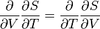
When the inexact differential DW is divided by p, the quantity DW/p becomes obviously equal to the differential dV of the differentiable state function V. State functions depend only on the actual values of the thermodynamic parameters (they depend on a single point in state space, a state function is local in state space). A state function does not depend on the points on the path along which the state was reached (the history of the state). Mathematically this means that integration from point 1 to point 2 along path I in state space is equal to integration along a different path II,

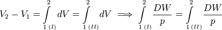
$V_2 - V_1 = {\int\limits_1\limits^2}_{{\!\!}^{(I)}} dV = {\int\limits_1\limits^2}_{{\!\!}^{(II)}} dV \;\Longrightarrow\; {\int\limits_1\limits^2}_{{\!\!}^{(I)}} \frac{DW}{p} = {\int\limits_1\limits^2}_{{\!\!}^{(II)}} \frac{DW}{p}$

The amount of work (divided by p) performed reversibly along path I is equal to the amount of work (divided by p) along path II. This condition is necessary and sufficient that DW/p is the differential of a state function. So, although DW is not a differential, the quotient DW/p is one.

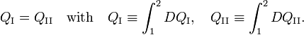
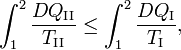
Reversible absorption of a small amount of heat DQ is another energy contact of a system with its surroundings; DQ is again not a differential of a certain function. In a completely analogous manner to DW/p, the following result can be shown for the heat DQ (divided by T) absorbed reversibly by the system along two different paths (along both paths the absorption is reversible):

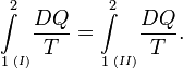
${\int\limits_1\limits^2}_{{\!\!}^{(I)}}\frac{DQ}{T} = {\int\limits_1\limits^2}_{{\!\!}^{(II)}} \frac{DQ}{T} .$

(1)

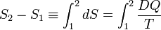
Hence the quantity dS defined by

$dS \;\stackrel{\mathrm{def}}{=}\; \frac{DQ}{T}$

is the differential of a state variable S, the entropy of the system. In the next subsection equation (1) will be proved from the Kelvin-Planck principle. Observe that this definition of entropy only fixes entropy differences:

$S_2-S_1 \equiv \int_1^2 dS = \int_1^2 \frac{DQ}{T}$

Note further that entropy has the dimension energy per degree temperature (joule per degree kelvin) and recalling the first law of thermodynamics (the differential dU of the internal energy satisfies dU = DQ − DW), it follows that

$dU = TdS - pdV.\,$

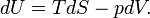
(For convenience sake only a single work term was considered here, namely DW = pdV, work done by the system). The internal energy is an extensive quantity. The temperature T is an intensive property, independent of the size of the system. It follows that the entropy S is an extensive property. In that sense the entropy resembles the volume of the system. We reiterate that volume is a state function with a well-defined mechanical meaning, whereas entropy is introduced by analogy and is not easily visualized. Indeed, as is shown in the next subsection, it requires a fairly elaborate reasoning to prove that S is a state function, i.e., that equation (1) holds.

[edit] Proof that entropy is a state function

Equation (1) gives the sufficient condition that the entropy S is a state function. The standard proof of equation (1), as given now, is physical, by means of an engine making Carnot cycles, and is based on the Kelvin-Planck formulation of the second law of thermodynamics.

Consider the figure. A system, consisting of an arbitrary closed system C (only heat goes in and out) and a reversible heat engine E, is coupled to a large heat reservoir R of constant temperature T₀. The system C undergoes a cyclic state change 1-2-1. Since no work is performed on or by C, it follows that

$Q_\mathrm{I} =Q_\mathrm{II} \quad\hbox{with}\quad Q_\mathrm{I} \equiv \int_1^2 DQ_\mathrm{I},\quad Q_\mathrm{II} \equiv \int_1^2 DQ_\mathrm{II}.$

For the heat engine E it holds (by the definition of thermodynamic temperature) that

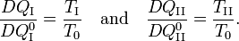
$\frac{DQ_\mathrm{I}}{DQ^0_\mathrm{I}} = \frac{T_\mathrm{I}}{T_0}\quad\hbox{and}\quad \frac{DQ_\mathrm{\mathrm{II}}}{DQ^0_\mathrm{II}} = \frac{T_\mathrm{II}}{T_0} .$

Hence

$\frac{Q^0_\mathrm{I}}{T_0} \equiv \frac{1}{T_0} \int_1^2 DQ^0_\mathrm{I} = \int_1^2 \frac{DQ_\mathrm{I}}{T_\mathrm{I}} \quad\hbox{and}\quad \frac{Q^0_\mathrm{II}}{T_0} \equiv \frac{1}{T_0} \int_1^2 DQ^0_\mathrm{II} = \int_1^2 \frac{DQ_\mathrm{II}}{T_\mathrm{II}} .$

From the Kelvin-Planck principle it follows that W is necessarily less or equal zero, because there is only the single heat source R from which W is extracted. Invoking the first law of thermodynamics we get,

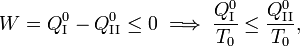
$W = Q^0_\mathrm{I} - Q^0_\mathrm{II} \le 0\; \Longrightarrow\; \frac{Q^0_\mathrm{I}}{T_0} \le \frac{Q^0_\mathrm{II}}{T_0},$

so that

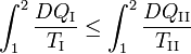
$\int_1^2 \frac{DQ_\mathrm{I}}{T_\mathrm{I}} \le \int_1^2 \frac{DQ_\mathrm{II}}{T_\mathrm{II}}$

Because the processes inside C and E are assumed reversible, all arrows can be reverted and in the very same way it is shown that

$\int_1^2 \frac{DQ_\mathrm{II}}{T_\mathrm{II}} \le \int_1^2 \frac{DQ_\mathrm{I}}{T_\mathrm{I}},$

so that equation (1) holds (with a slight change of notation, subscripts are transferred to the respective integral signs):

${\int\limits_1\limits^2}_{{\!\!}^{(I)}}\frac{DQ}{T} = {\int\limits_1\limits^2}_{{\!\!}^{(II)}} \frac{DQ}{T} .$

[edit] Relation to Gibbs free energy and enthalpy

The definition of Gibbs free energy is based on entropy as follows:

$G = H - T S\;$

where all the thermodynamic properties except T are extensive and where

G = Gibbs free energy

H = enthalpy

T = absolute temperature

S = entropy

A corresponding equation with all intensive properties (i.e., per unit of mass) can be written as follows:

$g = h - T s\;$

where

g = specific Gibbs free energy

h = specific enthalpy

T = absolute temperature

S = specific entropy

[edit] Entropy of an ideal gas

The equation of state of one mole of an ideal gas is

$pV = RT, \qquad \qquad\qquad\qquad\qquad \qquad\qquad\qquad\qquad \qquad\qquad\qquad\qquad (\mathrm{E1})$

where R is the molar gas constant, p the pressure, and V the volume of the gas. Note that the limit T → 0 implies V → 0—ideal-gas particles are of zero size.

The entropy of one mole of an ideal gas is a function of T and V and depends parametrically on the molar gas constant R and the molar heat capacity at constant volume, C_V,

$S(T,V) = C_V \log(T) + R \log(V) + S_0=R\log( T^{\frac{C_V}{R}}\, V) + S_0,$

where S₀ is a constant independent of T, V, and p. From statistical thermodynamics it is known that for an atomic ideal gas C_V = 3R/2, so that the exponent of T becomes 3/2. For a diatomic ideal gas C_V = 5R/2 and for an ideal gas of arbitrarily shaped molecules C_V = 3R. In any case, for an ideal gas C_V is constant, independent of T, V, or p.

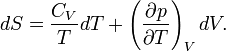
The expression for the ideal gas entropy is derived easily by substituting the ideal gas law (E1) into the following general differential equation for the entropy as function of T and V—valid for any thermodynamic system,

$dS = \frac{C_V}{T} dT + \left(\frac{\partial p}{\partial T}\right)_V dV.\qquad \qquad\qquad \qquad\qquad\qquad \qquad\qquad \qquad\qquad(\mathrm{E2}).$

Integration gives

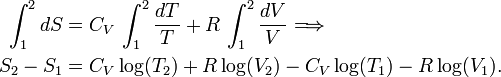
$\begin{align} \int_1^2 dS &= C_V\, \int_1^2 \frac{dT}{T} + R\, \int_1^2 \frac{dV}{V}\Longrightarrow \\ S_2-S_1 &= C_V\log(T_2) + R \log(V_2) -C_V \log(T_1) -R\log(V_1) . \end{align}$

Write

$S_0 \equiv S_1 -C_V \log(T_1) -R\log(V_2) \quad\hbox{and}\quad S_2 \equiv S,\; T_2\equiv T,\, V_2\equiv V$

and the result follows.

[edit] Proof of differential equation for S(T,V)

The proof of the differential equation (E2) follows by some typical classical thermodynamics calculus.

First, the internal energy at constant volume follows thus,

$dU = \left(\frac{\partial U}{\partial T}\right)_V dT + \left(\frac{\partial U}{\partial V}\right)_T dV\; \underset{\scriptstyle\mathrm{constant}\; V} {\Longrightarrow}\; dU = \left(\frac{\partial U}{\partial T}\right)_V dT .$

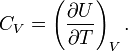
The definition of heat capacity and the first law (DQ = dU+pdV, for constant volume: DQ=dU) give,

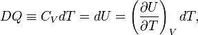
$DQ \equiv C_V dT = dU = \left(\frac{\partial U}{\partial T}\right)_V dT,$

so that the heat capacity at constant volume is given by

$C_V = \left(\frac{\partial U}{\partial T}\right)_V.$

The first and second law combined (TdS=dU+pdV) gives

$dS = \underbrace{\frac{C_V}{T}}_{\frac{\partial S}{\partial T}} dT + \underbrace{\frac{1}{T} \left[\left(\frac{\partial U}{\partial V}\right)_T + p\right]}_{\frac{\partial S}{\partial V}} dV. \qquad\qquad\qquad\qquad\qquad\qquad\qquad(\mathrm{E}3)$

From,

$\frac{\partial}{\partial V} \frac{\partial S}{\partial T} = \frac{\partial}{\partial T} \frac{\partial S}{\partial V}$

and

$\frac{\partial}{\partial V} \frac{\partial S}{\partial T} = \frac{\partial}{\partial V}\frac{C_V}{T} = \frac{1}{T} \frac{\partial C_V}{\partial V} = \frac{1}{T} \frac{\partial^2 U}{\partial V\partial T}$

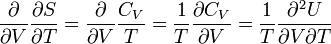
and

$\frac{\partial}{\partial T} \frac{\partial S}{\partial V} = \frac{\partial}{\partial T} \frac{1}{T} \left[\left( \frac{\partial U}{\partial V} \right)_T + p\right] = -\frac{1}{T^2} \left[ \left(\frac{\partial U}{\partial V}\right)_T +p\right] + \frac{1}{T}\left[ \left(\frac{\partial^2 U}{\partial T\partial V}\right)+\left(\frac{\partial p}{\partial T}\right)_V \right]$

follows

$0 = -\frac{1}{T^2} \left[ \left(\frac{\partial U}{\partial V}\right)_T +p\right] + \frac{1}{T} \left(\frac{\partial p}{\partial T}\right)_V \Longrightarrow \left(\frac{\partial U}{\partial V}\right)_T = -p + T \left(\frac{\partial p}{\partial T}\right)_V.$

Substitute the very last equation into equation (E3), and the equation to be proved follows,

$dS = \frac{C_V}{T} dT + \left(\frac{\partial p}{\partial T}\right)_V dV.$

[edit] Entropy in statistical thermodynamics

In classical (phenomenological) thermodynamics it is not necessary to assume that matter consists of small particles (atoms or molecules). While this has the advantage of keeping classical thermodynamics transparent, not obscured by microscopic details, and universally valid, independent of the kind of molecules constituting the system, it has the disadvantage that it cannot predict the value of any parameters. For instance, the heat capacity of a monoatomic ideal gas at constant volume C_V is equal to 3R/2, where R is the molar gas constant. One needs a microscopic theory to find this simple result.

The Boltzmann equation is engraved on Boltzmann's tombstone.^[12]

Before the 1920s the microscopic (molecular) theory of thermodynamics was based on classical (Newtonian) mechanics and on the kind of statistical arguments that were first introduced into physics by Maxwell and developed by Gibbs and Boltzmann. The branch of physics that tries to predict thermodynamic properties departing from molecular properties is known as statistical thermodynamics or statistical mechanics. Since the 1920s statistical thermodynamics is based usually on quantum mechanics.

In this section it will be shown that the statistical mechanics expression for the entropy is

$S = - k_\mathrm{B} \mathrm{Tr}[\hat{\rho} \log {\hat{\rho}}]$

where the density operator $\hat{\rho}$ is given by

$\hat{\rho} = \frac{ e^{-\hat{H}/(k_\mathrm{B}T)} }{ \mathrm{Tr}[ e^{-\hat{H}/(k_\mathrm{B}T)}] }.$

Further k_B is Boltzmann's constant, Ĥ is the quantum mechanical energy operator of the total system (the energies of all particles plus their interactions), and the trace (Tr) of an operator is the sum of its diagonal matrix elements.

It will also be shown under which circumstance the entropy may be given by Boltzmann's celebrated equation

$S = k \log W.\,$

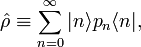
[edit] Density operator

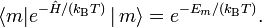
In his book^[6]John von Neumann introduced into quantum mechanics the density operator $\hat{\rho}$ (called "statistical operator" by von Neumann) for a system of which the state is only partially known. He considered the situation that certain real numbers p_m are known that correspond to a complete set of orthonormal quantum mechanical states (m = 0, 1, 2, …, ∞).^[13] The quantity p_m is the probability that state |m⟩ is occupied, or in other words, it is the percentage of systems in a (very large) ensemble of identical systems that are in the state |m⟩. As is usual for probabilities, they are normalized to unity,

$\sum_{m=0}^\infty p_m = 1.$

The averaged value of a property with quantum mechanical operator $\hat{P}$ of a system described by the probabilities p_m is given by the ensemble average,

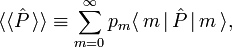
$\langle\langle\hat{P}\, \rangle\rangle \equiv \sum_{m=0}^\infty p_m \langle\, m\,|\, \hat{P} \,|\,m\,\rangle ,$

where $\langle m |\hat{P}\,|m\rangle$ is the usual quantum mechanical expectation value.

The expression for ⟨⟨P ⟩⟩ can be written as a trace of an operator product. First define the density operator;

$\hat{\rho} \equiv \sum_{n=0}^\infty | n\rangle p_n \langle n| ,$

then it follows that

$\langle\langle \hat{P}\, \rangle\rangle = \mathrm{Tr}\big[ \hat{P}\hat{\rho}\big].$

Indeed,

$\begin{align} \mathrm{Tr}\left[ \hat{P}\,\hat{\rho}\,\right] &\equiv \sum_m \langle m \,|\hat{P}\,\hat{\rho}\,| m\,\rangle = \sum_{nm} \langle\, m \,|\,n\rangle\, p_n\,\langle\, n| \hat{P}\,|\, m\,\rangle =\sum_{nm} p_n \delta_{mn} \langle n\,|\, \hat{P}\,|\, m\rangle \\ &= \sum_m p_m \langle m\,|\, \hat{P}\,|\, m\rangle = \langle\langle \hat{P}\, \rangle\rangle, \end{align}$

where ⟨ m | n ⟩ = δ_mn, the Kronecker delta.

A density operator has unit trace

$\mathrm{Tr}\hat{\rho} = \sum_{mn} \langle m\,|\, n\rangle\,p_n\,\langle n \,|\, m\rangle= \sum_n p_n \sum_{m}\delta_{nm}\delta_{mn} = \sum_n p_n \delta_{nn} = \sum_n p_n = 1.$

[edit] Closed isothermal system

For a thermodynamic system of constant temperature (T), volume (V), and number of particles (N),one considers eigenstates of the energy operator $\hat{H}$ , the Hamiltonian of the total system,

$\hat{H} \, |\,m\rangle = E_m \, |\,m\rangle.$

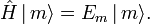
Assume that p_m is proportional to the Boltzmann factor, with the proportionality constant K determined by normalization,

$p_m = K e^{-E_m/(k_\mathrm{B} T)}\quad \hbox{with} \quad K\sum_m e^{-E_m/(k_\mathrm{B} T)} = 1 \Longrightarrow K = \left[ \sum\limits_m e^{-E_m/(k_\mathrm{B} T)}\right]^{-1},$

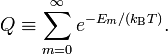
where k_B is the Boltzmann constant. It is common to designate the partition function of the system of constant T, N, and V by Q,

$Q \equiv \sum_{m=0}^\infty e^{-E_m/(k_\mathrm{B} T)}.$

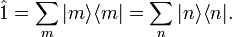
Hence, using that

$\langle m| e^{-\hat{H}/(k_\mathrm{B} T)} \, |\,m\rangle = e^{-E_m/(k_\mathrm{B} T)} .$

it is found

$\hat{\rho} =\frac{1}{Q}\sum_m |m\rangle \langle m| e^{-\hat{H}/(k_\mathrm{B} T)} \, |\,m\rangle \langle m| = \frac{1}{Q}\sum_{mn} |m\rangle \langle m| e^{-\hat{H}/(k_\mathrm{B} T)} \, |\,n\rangle \langle n| = \frac{\exp[-\hat{H}/(k_\mathrm{B} T)]}{Q},$

where it used that the set of states is complete—give rise to the following resolution of the identity operator,

$\hat{1} = \sum_m |m\rangle \langle m| = \sum_n |n\rangle \langle n| .$

In summary, the canonical ensemble^[14] average of a property with quantum mechanical operator $\hat{P}$ is given by

$\langle\langle \hat{P}\, \rangle\rangle = \mathrm{Tr}\big[ \hat{P}\hat{\rho}\big] = \frac{1}{Q}\mathrm{Tr}\big[ \hat{P} e^{-\hat{H}/(k_\mathrm{B} T)} \big].$

[edit] Internal energy

The quantum statistical expression for internal energy is

$U \equiv \langle\langle \hat{H}\, \rangle\rangle = \mathrm{Tr}\big[ \hat{H}\hat{\rho}\big] = \frac{1}{Q}\mathrm{Tr}\big[ \hat{H} e^{-\hat{H}/(k_\mathrm{B} T)} \big].$

From

$\log\hat{\rho} = \log \big[ e^{-\hat{H}/(k_\mathrm{B} T)}/Q \big] = -\hat{H}/(k_\mathrm{B} T) - \hat{1}\,\log Q$

follows

$\hat{H} = -k_\mathrm{B} T \big( \log\hat{\rho} + \hat{1}\log Q \big).$

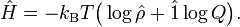
The quantum statistical expression for the internal energy U becomes

$U= \mathrm{Tr}\left[ -k_\mathrm{B} T \big( \log\hat{\rho} + \hat{1}\log Q \big) \hat{\rho}\right] = - T\; k_\mathrm{B}\;\mathrm{Tr}[\hat{\rho}\log\hat{\rho}] - T \;k_\mathrm{B}\;\log(Q),$

where it is used that a scalar may be taken of the trace and that the density operator is of unit trace.

In classical thermodynamics the internal energy is related to the entropy S and the Helmholtz free energy A by

$U = T\,S + A.$

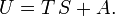
Define

$\hat{S} \equiv - k_\mathrm{B}\, \log\hat{\rho}, \quad \hat{A} \equiv -k_\mathrm{B}\,T\,\log(Q) \,\hat{1} \qquad\qquad\qquad\qquad(\mathrm{S1})$

and accordingly

$S \equiv \langle\langle \hat{S}\, \rangle\rangle = \mathrm{Tr}[\hat{S}\hat{\rho}] = - k_\mathrm{B}\,\mathrm{Tr}[\hat{\rho} \log\hat{\rho} ]$

and

$A \equiv \langle\langle \hat{A}\, \rangle\rangle =-\mathrm{Tr}[\hat{A}\hat{\rho}] = -k_\mathrm{B}\,T\; \log(Q)\mathrm{Tr}[ \hat{\rho}] = - k_\mathrm{B}\,T\; \log(Q).$

In summary,

$U = TS + A = - k_\mathrm{B}\,T\, \mathrm{Tr}[\hat{\rho} \log\hat{\rho} ] - k_\mathrm{B}\,T\; \log(Q),$

which agrees with the quantum statistical expression for U, which in turn means that the definitions (S1) of the entropy operator and Helmholtz free energy operator are consistent.

Note that neither the entropy nor the free energy are given by an ordinary quantum mechanical operator, both depend on the temperature through the partition function Q. Furthermore Q is defined as a trace:

$Q = \mathrm{Tr}[ e^{-\hat{H}/(k_\mathrm{B}\,T)} ]$

and thus samples the whole (Hilbert) space containing the state vectors | m ⟩. Almost all quantum mechanical operators that represent observable (physical) quantities have a classical (electromagnetic or mechanical) counterpart. Clearly the entropy operator lacks such a parallel definition, and this is probably the main reason why entropy is a concept that is difficult to comprehend

[edit] Boltzmann's formula for entropy

Let us consider an isolated system (constant U, V, and N). Traces are taken only over states with energy U. Let there be Ω(U, V, N) of these states. This is in general a very large number, for instance for one mole of a mono-atomic ideal gas consisting of N = N_A ≈ 10²³ (Avogadro's number) it holds that^[15]

$\Omega(U, V, N) = \left[ \left( \frac{2\pi m k_\mathrm{B}T}{h^2} \right)^{3/2} \frac{V e^{5/2}}{N^{5/2}}\right]^N \approx e^{N} \approx 10^{10^{23}}.$

Here m is the mass of an atom, h is Planck's constant, V is the volume of the vessel containing the gas, and e ≈ 2.7.

The sum in the partition function shrinks to a sum over Ω states of energy U, hence

$Q = \mathrm{Tr}\big[ e^{-\hat{H}/(k_\mathrm{B}T)} \big] = \Omega(U,V,N) e^{-U/(k_\mathrm{B}T)}.$

Likewise,

$S = - k_\mathrm{B} \mathrm{Tr} \rho \log\rho = - k_\mathrm{B} \Omega \frac{e^{-U/(k_\mathrm{B}T)}}{Q} \log\left(\frac{e^{-U/(k_\mathrm{B}T)}}{Q}\right) = - k_\mathrm{B} \log \frac{1}{\Omega},$

so that Boltzmann's celebrated equation follows^[12]

$S = k_\mathrm{B} \log\Omega(U,V,N). \,$

From the previous expression for Ω follows an expression for the entropy of a mono-atomic ideal gas as a function of T and V,

$S = Nk_\mathrm{B} \log(V\, T^{3/2}) + S_0\quad\hbox{with}\quad S_0 = Nk_\mathrm{B} \log\left[ \left( \frac{2\pi m k_\mathrm{B}}{h^2} \right)^{3/2} \frac{e^{5/2}}{N^{5/2}}\right].$

Recalling that N_Ak_B ≡ R and C_V = 3/2 R one sees that this is the formula encountered above [between Eqs. (E1) and (E2)], but this time with an explicit expression for S₀.

Boltzmann's equation is derived as an average over an ensemble consisting of identical systems of constant energy, number of particles, and volume; such an ensemble is known as a microcanonical ensemble. However, it can be shown that energy fluctuations around the mean energy in a canonical ensemble (constant T) are extremely small, so that taking the trace over only the states of mean energy is a very good approximation. In other words, although Boltzmann's formula does not hold formally for a canonical ensemble, in practice it is a very good approximation, also for isothermal systems.

[edit] Entropy as disorder

In common parlance the term entropy is used for lack of order and gradual decline into disorder. One can find in many introductory physics texts the statement that entropy is a measure for the degree of randomness in a system.

The origin of these statements is Boltzmann's 1877 equation S=k_B logΩ that was discussed above. The third law of thermodynamics states the following: when T → 0 the number of accessible states Ω goes to unity, and the entropy S goes to zero. That is, if one interprets entropy as randomness, then at zero K there is no disorder whatsoever, matter is in complete order. Clearly, this low-temperature limit supports the intuitive notion of entropy as a measure of chaos.

It was shown above that Ω gives the number of quantum states accessible to a system. It can be argued that the more quantum states are available to a system, the greater the complexity of the system. If one equates complexity with randomness, as is often done in this context, it confirms the notion of entropy as a measure of disorder. The second law of thermodynamics, which states that a spontaneous process in an isolated system strives toward maximum entropy, can be interpreted as the tendency of the universe to become more and more chaotic.

However, the view of entropy as disorder, as a measure of chaos, is disputed. For instance, Lambert^[16] contends that entropy is a "measure for energy dispersal". If one reads "energy dispersal" as heat divided by temperature, this is true by the classical (phenomenological) definition of entropy. Lambert states that from a molecular point of view, entropy increases when more microstates become available to the system (i.e., Ω increases) and the energy is dispersed over the greater number of accessible microstates. This interpretation agrees with the discussion above. Lambert argues further that the view of entropy as disorder, is "so misleading as actually to be a failure-prone crutch".

If one rejects completely the idea of entropy as randomness, one discards a convenient mnemonic device. Generations of physicists and chemists have remembered that a gas contains more entropy than a crystal, "because a gas is more chaotic than a crystal". This is easier to remember than "because the gas has more microstates to its disposal and its energy is dispersed over these larger number of microstates", although the latter statement is the more correct one.

[edit] Entropy as function of aggregation state

As just stated, the entropy of a mole of pure substance changes as follows

S_gas > S_liq > S_sol

which agrees with our intuition that a gas is more chaotic than a liquid, which again is more chaotic than a solid.

As an illustration of this point, consider one mole of water (H₂O) at a pressure of 1 bar (≈ 1 atmosphere). Experimentally, the enthalpy of fusion ΔH_f is 6.01 kJ/mol and the enthalpy of vaporization ΔH_v is 40.72 kJ/mol. Remember that enthalpy is heat added/extracted reversibly at constant pressure (in this case 1 bar) to achieve the change of aggregation state. Further the change of aggregation state occurs at constant temperature, so that

$\Delta S_\textrm{f} = \frac{\Delta H_\textrm{f}}{T_\textrm{f}} \quad\hbox{and}\quad \Delta S_\textrm{v} = \frac{\Delta H_\textrm{v}}{T_\textrm{v}}.$

For water T_f = 0 °C = 273.15 K and T_v = 100 °C = 373.15 K. Hence

$\Delta S_\textrm{f} = 22.0\; \mathrm{J/(mol\; K)}\quad\hbox{and}\quad \Delta S_\textrm{v} = 109.1 \;\mathrm{J/(mol\; K)}.$

Summarizing, in units J/(mol K) a mole of liquid water contains 22.0 more entropy than a mole of ice (both at 0 °C); a mole of gas (steam at 100 °C) contains 109.1 more entropy than a mole of liquid water at boiling temperature.

[edit] Footnotes

↑ A size-extensive property of a system becomes x times larger when the system is enlarged by a factor x, provided all intensive parameters remain the same upon the enlargement. Intensive parameters, like temperature, density, and pressure, are independent of size.
↑ It is reported that in a conversation with Claude Shannon, John (Johann) von Neumann said: "In the second place, and more important, nobody knows what entropy really is [..]”. M. Tribus, E. C. McIrvine, Energy and information, Scientific American, vol. 224 (September 1971), pp. 178–184.
↑ ^3.0 ^3.1 R. J. E. Clausius, Ueber verschiedene für die Anwendung bequeme Formen der Hauptgleichungen der Mechanischen Wärmetheorie [On several forms of the fundamental equations of the mechanical theory of heat that are useful for application], Annalen der Physik, (is Poggendorff's Annalen der Physik und Chemie) vol. 125, pp. 352–400 (1865) pdf. Around the same time Clausius wrote a two-volume treatise: R. J. E. Clausius, Abhandlungen über die mechanische Wärmetheorie [Treatise on the mechanical theory of heat], F. Vieweg, Braunschweig, (vol I: 1864, vol II: 1867); Google books (contains two volumes). The 1865 Annalen paper was reprinted in the second volume of the Abhandlungen and included in the 1867 English translation.
↑ S. Carnot, Réflexions sur la puissance motrice du feu et sur les machines propres à développer cette puissance (Reflections on the motive power of fire and on machines suited to develop that power), Chez Bachelier, Paris (1824).
↑ L. Boltzmann, Über die Beziehung zwischen dem zweiten Hauptsatz der mechanischen Wärmetheorie und der Wahrscheinlichkeitsrechnung respektive den Sätzen über das Wärmegleichgewicht, [On the relation between the second fundamental law of the mechanical theory of heat and the probability calculus with respect to the theorems of heat equilibrium] Wiener Berichte vol. 76, pp. 373-435 (1877)
↑ ^6.0 ^6.1 J. von Neumann, Mathematische Grundlagen der Quantenmechanik, [Mathematical foundation of quantum mechanics] Springer, Berlin (1932)
↑ C. Carathéodory, Untersuchungen über die Grundlagen der Thermodynamik [Investigation on the foundations of thermodynamics], Mathematische Annalen, vol. 67, pp. 355-386 (1909).
↑ M. Born, Physikalische Zeitschrift, vol. 22, p. 218, 249, 282 (1922)
↑ H. B. Callen, Thermodynamics and an Introduction to Thermostatistics. John Wiley and Sons, New York, 2nd edition, (1965)
↑ E. A. Guggenheim, Thermodynamics, North-Holland, Amsterdam, 5th edition (1967)
↑ ^11.0 ^11.1 H. Reiss, Methods of Thermodynamics, Dover (1996).
↑ ^12.0 ^12.1 The equation S = k log W is engraved on the tombstone of the Ehrengrab (grave of honour) in Vienna (Wiener Zentralfriedhof, Ehrengräber Gruppe 14C Nummer 1).
↑ In order to distinguish the macroscopic thermodynamical states of a system (determined by a few thermodynamic parameters, such as T and V) from the quantum mechanical states (functions of 3N parameters, the coordinates of the N particles), the quantum mechanical states are often referred to as "microstates".
↑ A large number of systems with constant T, V, and N is known as a canonical ensemble; the term is due to Willard Gibbs.
↑ T. L. Hill, An introduction to statistical thermodynamics, Addison-Wesley, Reading, Mass. (1960) p. 82
↑ F. L. Lambert, Disorder—A Cracked Crutch for Supporting Entropy Discussions, Journal of Chemical Education, vol. 79 pp. 187–192 (2002)

[edit] References

M. W. Zemansky, Kelvin and Carathéodory—A Reconciliation, American Journal of Physics Vol. 34, pp. 914-920 (1966) [1]

[0] A size-extensive property of a system becomes x times larger when the system is enlarged by a factor x, provided all intensive parameters remain the same upon the enlargement. Intensive parameters, like temperature, density, and pressure, are independent of size.

[1] It is reported that in a conversation with Claude Shannon, John (Johann) von Neumann said: "In the second place, and more important, nobody knows what entropy really is [..]”. M. Tribus, E. C. McIrvine, Energy and information, Scientific American, vol. 224 (September 1971), pp. 178–184.

[Clausius1865-2] 3.0 ^3.1 R. J. E. Clausius, Ueber verschiedene für die Anwendung bequeme Formen der Hauptgleichungen der Mechanischen Wärmetheorie [On several forms of the fundamental equations of the mechanical theory of heat that are useful for application], Annalen der Physik, (is Poggendorff's Annalen der Physik und Chemie) vol. 125, pp. 352–400 (1865) pdf. Around the same time Clausius wrote a two-volume treatise: R. J. E. Clausius, Abhandlungen über die mechanische Wärmetheorie [Treatise on the mechanical theory of heat], F. Vieweg, Braunschweig, (vol I: 1864, vol II: 1867); Google books (contains two volumes). The 1865 Annalen paper was reprinted in the second volume of the Abhandlungen and included in the 1867 English translation.

[3] S. Carnot, Réflexions sur la puissance motrice du feu et sur les machines propres à développer cette puissance (Reflections on the motive power of fire and on machines suited to develop that power), Chez Bachelier, Paris (1824).

[4] L. Boltzmann, Über die Beziehung zwischen dem zweiten Hauptsatz der mechanischen Wärmetheorie und der Wahrscheinlichkeitsrechnung respektive den Sätzen über das Wärmegleichgewicht, [On the relation between the second fundamental law of the mechanical theory of heat and the probability calculus with respect to the theorems of heat equilibrium] Wiener Berichte vol. 76, pp. 373-435 (1877)

[Von_Neumann-5] 6.0 ^6.1 J. von Neumann, Mathematische Grundlagen der Quantenmechanik, [Mathematical foundation of quantum mechanics] Springer, Berlin (1932)

[6] C. Carathéodory, Untersuchungen über die Grundlagen der Thermodynamik [Investigation on the foundations of thermodynamics], Mathematische Annalen, vol. 67, pp. 355-386 (1909).

[7] M. Born, Physikalische Zeitschrift, vol. 22, p. 218, 249, 282 (1922)

[8] H. B. Callen, Thermodynamics and an Introduction to Thermostatistics. John Wiley and Sons, New York, 2nd edition, (1965)

[9] E. A. Guggenheim, Thermodynamics, North-Holland, Amsterdam, 5th edition (1967)

[Reiss-10] 11.0 ^11.1 H. Reiss, Methods of Thermodynamics, Dover (1996).

[Grave-11] 12.0 ^12.1 The equation S = k log W is engraved on the tombstone of the Ehrengrab (grave of honour) in Vienna (Wiener Zentralfriedhof, Ehrengräber Gruppe 14C Nummer 1).

[12] In order to distinguish the macroscopic thermodynamical states of a system (determined by a few thermodynamic parameters, such as T and V) from the quantum mechanical states (functions of 3N parameters, the coordinates of the N particles), the quantum mechanical states are often referred to as "microstates".

[13] A large number of systems with constant T, V, and N is known as a canonical ensemble; the term is due to Willard Gibbs.

[14] T. L. Hill, An introduction to statistical thermodynamics, Addison-Wesley, Reading, Mass. (1960) p. 82

[15] F. L. Lambert, Disorder—A Cracked Crutch for Supporting Entropy Discussions, Journal of Chemical Education, vol. 79 pp. 187–192 (2002)

[1]

[2]

[3]

[4]

[5]

[6]

[7]

[8]

[9]

[10]

[11]

[12]

[13]

[14]

[15]

[16]

Entropy (thermodynamics)

Contents

[edit] Specific entropy

[edit] Traditional definition of entropy

[edit] Proof that entropy is a state function

[edit] Relation to Gibbs free energy and enthalpy

[edit] Entropy of an ideal gas

[edit] Proof of differential equation for S(T,V)

[edit] Entropy in statistical thermodynamics

[edit] Density operator

[edit] Closed isothermal system

[edit] Internal energy

[edit] Boltzmann's formula for entropy

[edit] Entropy as disorder

[edit] Entropy as function of aggregation state

[edit] Footnotes

[edit] References

Personal tools

Namespaces

Variants

Views

Actions

Search

Navigation

Community

Toolbox