Vacuum Techniques
In this experiment you will learn about vacuum technology and how to use it for measurements.
Experimental procedure
Determine the atmospheric pressure by measuring the force needed to open the vacuum system
- Build the illustrated system:
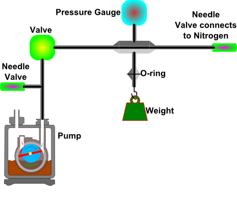
Figure 1a: Schematic illustration of the system to be built to measure the force needed to open the vacuum system. 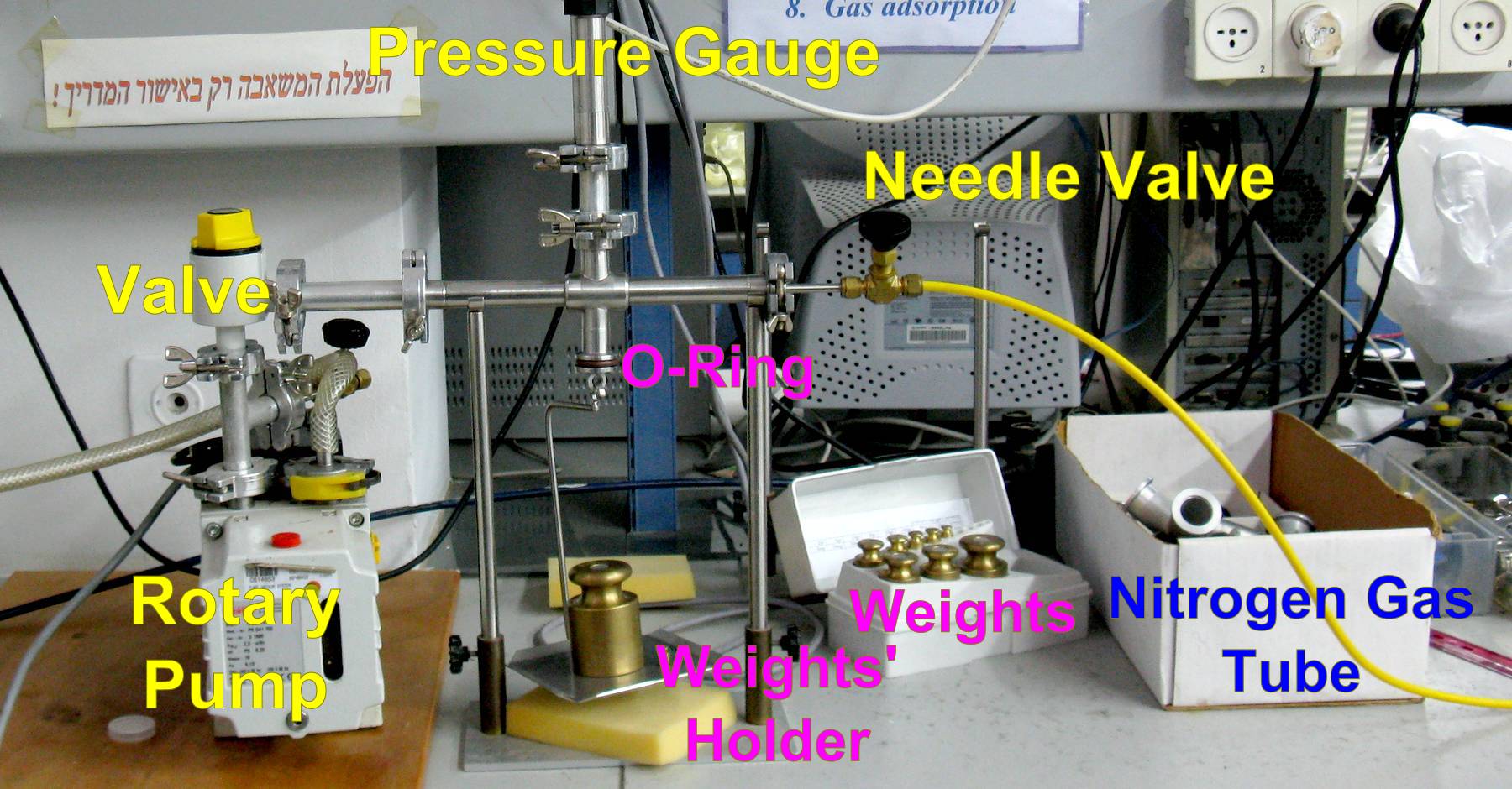
Figure 1b: Photograph of the same system illustrated in Figure 1a. - Hold the weight holder, and press it against the O-ring.
- Pump the air from the system, making sure that none of the connectors leak.
- Once the system is under reduced pressure, close the valve connecting the system to the pump.
- Calculate the expected pressure in which the weight will disconnect before performing the experiment.
Weight [gr] Weight Error [mg] Pressure 1000 290 --- 500 100 --- 100 30 --- 50 30 --- 20 20 --- 10 20 --- 5 10 --- - Let the nitrogen flow slowly through the needle valve that is directly connected to the vacuum system until the weight falls. Monitor the pressure of the system and record the pressure immediately before the weight falls. Based on this first measurement and your calculation, what are likely sources of error in this experiment? Estimate their values and write them down.
- Repeat this experiment for several weights.
- Fill in the table and plot (in the correct units) pressure versus total weight. Find the atmospheric pressure and find the O-ring sealing area.
| Total Weight | Pressure |
|---|---|
| --- | --- |
Measurement of pumping speed of the rotary pump when volume is fixed
- Build the system illustrated in Figure 2. Notice that you should build your system as large as possible (why should you do this?). Before building the system, measure the dimensions of all components so that you can estimate your system volume via direct measurements.
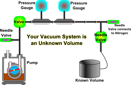
Figure 2a: Schematic illustration of the system to be built to measure the pumping speed of the rotary pump when the volume is fixed. 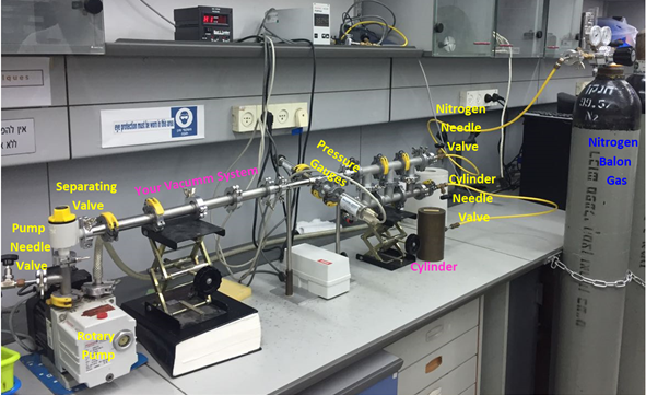
Figure 2b: Photograph of the same system illustrated in Figure 2a. - Make sure that both the Pirani and the Piezo pressure gauges are connected.
- In order to measure the pumping speed of the pump, you should first measure the volume of your system using a known volume. In this case, of the cylinder. Assuming the gases are ideal and moles are conserved, by the use of Boyle's law, the unknown pressure can be calculated by the expression:
The measurement process:
$P_{total} V_{total}=P_{known} V_{known} +P_{unknown} V_{unknown}$
$V_{total}=V_{known} + V_{unknown}$
$(P_{known}-P_{total})V_{known}=(P_{total}-P_{unknown})V_{unknown}$
- Construct the illustrated system and close all the valves. The system will be at atmospheric pressure.
- In order to measure the unknown volume of your system, you will need to measure both the pressure of your system (the unknown volume) and of the cylinder (the known volume), at every time that you open or close one of the valves.
- You can start either from atmospheric pressure or from vacuum. To start from vacuum, first pump down the entire system. Write down the pressure you obtained and its error as $P_{known}=P_{eq}^{(1)}$.
- o With the two parts of the system still separated : If you started from atmospheric pressure open the pump needle valve and pump down the unknown volume. If you started from vacuum, open the nitrogen needle valve and allow it to flow to the unknown volume. Close the needle valve that you opened. Write down the new pressure, $P_{unknown}^{(1)}$, and its error (note that the pressure in the cylinder is still $P_{eq}^{(1)}$).
- Open the valve separating the two parts of the system (the known and the unknown volumes) and wait until it stabilizes. Write down the pressure, $P_{total}=P_{eq}^{(2)}$, and its error.
- Close the valve separating the two parts and ether open the pump needle valve and pump down the unknown volume or open the nitrogen needle valve and allow it to flow to the unknown volume. As before take a measurement of the pressure in your system, $P_{unknown}^{(2)}$, and its error (note that the pressure in the cylinder is still $P_{eq}^{(2)}$).
- Repeat the process.
- You should fill the table (make sure the correct units are used):
$$P_{eq}$$ $$P_{unknown}$$ --- --- - Plot $P_{eq}$ versus $P_{unknown}$, and determine the volume of the system and its error.
- Compare this result to the estimated volume of your system based on measurements of components made at the beginning of the experiment.
- After you have measured the system volume, pump down the entire system and then close both the needle valve of the pump and the valve separating the two parts of the system.
- Allow nitrogen to flow only to your vacuum system and fill it until reaching atmospheric pressure. Do not pass the 1 atmosphere limit!.
- Begin taking a video of both the Pirani and the Piezo pressure gauges. Open the pump's needle valve and pump nitrogen out of the system. Note: The pressure gauges are connected and each gives a readout. Considering the gauges working pressure ranges and the dependence of the pumping speed on the pressure, is one of the gauges more correct (consider the measurement ranges provided by the manufacturer)? Which one? Monitor both readouts to defend your answer.
- Plot a graph that will allow you to calculate the pumping speed, S. Note that you should have at least one measurement per second. Compare your results to the manufacturer's value.
- Repeat steps 5-8, but this time, first open the valve separating the two parts of the system, and allow nitrogen to flow to the entire vacuum system until reaching atmospheric pressure. Compare the results.
Measurement of pumping speed of the rotary pump when pressure is fixed
- Disassmeble the system from the previous part and build a new system similiar to that illustrated at Figure 2a (without connecting your system to the known volume or to the Nitrogen gas source) and connect it to the mass flow meter (MFM). Make sure that the needle valve of the MFM is closed.
- In this part (and the following) use atmospheric pressure as your "source". Given that the pressure gauges are calibrated to measure nitrogen gas, will this affect the accuracy of readouts? Think carefully.
- Gently open the needle valve of the MFM and allow air to flow in. Wait for the reading to stabilize.
- Measure the pressure in your system and the rate of gas flow into your system. Be careful to take readings only from an instrument that is within range!
- Determine the pumping speed, S, and compare it to the value you obtained in the previous section. Compare your result to the manufacturer's value.
Measurement of conductivity of different tubes and calculation of the viscosity of air
Note: This part of the experiment is not currently performed. The corresponding theoretical material is retained for reference, but the procedure described below should be skipped. Please proceed instead to the next part: Measurement of the triple point of cyclohexane.
At your disposal there are tubes of different lengths and inner diameters.
- Build the system illustrated in Figure 3 with one of the tubes:
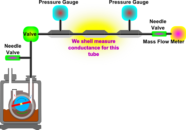
Figure 3: Schematic of system to be used to measure conductance of a tube. - Allow air to flow into the system via the needle valve connected to the MFM.
- Note the MFM reading and both of the pressure gauges readings. Make sure that you are in the linear range of all the gauges.
- Repeat this experiment with each tube. Fill the table below with your data (use the correct units).
Tube Diameter Tube Length SMass Flow Meter PGauge 1 PGauge 2 ----- ----- ----- ----- ----- ----- ----- ----- ----- ----- ----- ----- ----- ----- ----- ----- ----- ----- ----- ----- ----- ----- - Is it possible to determine the conductivity for each tube? What is the relavant equation?
- If not, why not?
- See equation 14, does the conductivity remain constant?
- Compare your results for conductivity of the tubes using equation (14). Take the air viscosity value from literature.
- What type of flow does eq.14 describe? Did you measure this type of flow?
- For each tube conductivity, you should be able to calculate the viscosity of the air. Compare the calculated air viscosity with the air viscosity value from literature.
- Using results obtained from experiments with different tubes, demonstrate that gas flow rate depends on the tube's diameter raised to the fourth power as stated in Poiseuille’s law (equation (13)). For this plot you will need to have at least five points (i.e., 5 measurements of tubes with the same length but different diameters).
Measurement of the triple point of cyclohexane
In this part of the experiment you will use a separate, dedicated apparatus to locate the triple point of cyclohexane — the unique combination of pressure and temperature at which solid, liquid, and vapor coexist in equilibrium. The strategy: set the temperature with a 6 °C water/ice bath, then approach the triple-point pressure of 40 Torr from above by slowly closing the MFM needle valve while the rotary pump pulls. With practice you can descend smoothly through 40 Torr and observe all three phases simultaneously inside the bulb for many seconds. Read the corresponding section of the theoretical background page before beginning, and make sure you understand the role of the cold trap and the meaning of the Gibbs phase rule (F = C - P + 2) at the triple point.
Safety: Cyclohexane is highly flammable (flash point about −20 °C). Keep the sample bulb away from open flames, hot plates, and any other source of ignition for the entire duration of the experiment. Work in a well-ventilated area.
Cold trap warning: The cold trap in this apparatus is the type that is filled with liquid nitrogen from above through a funnel, not the type that is lowered into an external Dewar. Never start filling the cold trap before the system is being pumped. Cooling an open trap will condense atmospheric oxygen as a pale blue liquid inside it, which is a serious explosion hazard in the presence of any organic residue. First start pumping, and only then carefully pour liquid nitrogen through the funnel into the trap. Add nitrogen slowly and steadily; the trap is full when you see liquid nitrogen begin to overflow from the top — that is your visual signal to stop pouring. Top up the trap as needed during the experiment so that it stays full.
- Build the system illustrated in Figure 6 of the theoretical background page (an actual photograph of the assembled system will be added in due course). The setup is a single chamber between the MFM (gas inlet) and the rotary pump. Verify that:
- All ground-glass joints are coated with a thin layer of vacuum grease and seated tightly.
- The pressure gauge is connected to the chamber.
- The Mass Flow Meter (MFM) is connected through its needle valve, and the needle valve is fully open at the start (so the chamber is freely open to the atmosphere through the MFM).
- The cold trap is mounted in line between the chamber and the rotary pump, but is still empty (no liquid nitrogen in it yet).
- The valve closest to the rotary pump is initially closed.
- Place the sample bulb in a water/ice bath at approximately 6 °C (close to the expected triple-point temperature of 6.32 °C). Allow the cyclohexane to equilibrate thermally with the bath for at least 5 minutes. Record the bath temperature using a calibrated thermometer.
- Turn on the rotary pump and open the valve closest to the pump. Because the MFM is fully open at the other end, atmospheric air flows smoothly through the chamber from MFM inlet to pump exhaust, and the chamber stays close to atmospheric pressure.
- Carefully fill the cold trap with liquid nitrogen using a funnel. Pour slowly and steadily until you see liquid nitrogen begin to overflow from the top of the trap — that is your visual signal that the trap is full. Stop pouring at that point. Plan to top up the trap a few minutes later, since the initial cooldown will boil off a substantial fraction of the nitrogen.
- Begin slowly closing the MFM needle valve. As you restrict the inflow of air, the pump pulls the chamber pressure down. Watch the pressure gauge and learn to control the rate of pressure decrease. This is a sensitive flow-balance: the chamber pressure at any instant is set by the equilibrium between MFM inflow and pump throughput. Closing the valve too quickly will cause the pressure to drop too fast and you will overshoot 40 Torr without seeing the triple point; closing too slowly will leave you at high pressure indefinitely. Aim for a smooth, controlled descent.
- ⚡ Question: Why do we expect the temperature of the sample to change as the pressure drops, even before the bath has had time to respond? (Hint: think about the latent heats of vaporization and sublimation discussed in the theoretical background.)
- Approach 40 Torr from above. As you continue closing the MFM, watch the pressure gauge and the sample bulb continuously. Slow your approach as you near 40 Torr so that you have time to observe the sample's response.
- Locate the triple point. As pressure passes through ~40 Torr at 6 °C, you should see vapor forming over the condensed phase, and — if your descent is slow and well-controlled enough — all three phases (solid, liquid, vapor) appearing simultaneously inside the bulb. The triple point is reached when these three phases are visible and remain stable for many seconds without one phase visibly disappearing in favor of another. The expected reading is approximately P = 40.4 Torr and T = 6.32 °C.
- Adjust the bath temperature in parallel as needed. Evaporative cooling at the surface of the sample tends to drag the bulb's temperature below the bath temperature; if you see the sample falling out of the triple-point regime because it has cooled too far, add small amounts of warm water to the bath to nudge it back toward 6.3 °C. Use the bath thermometer continuously.
- Record P and T at the triple point along with their estimated experimental uncertainties. Repeat the descent (steps 5–8) at least twice to assess reproducibility.
Step Phase(s) observed T [°C] ΔT P [Torr] ΔP Initial state (MFM open, atmospheric) solid only --- --- ~760 --- Approach (MFM closing, P descending) solid, vapor begins to appear --- --- --- --- Triple point (stable, several seconds) solid + liquid + vapor --- --- --- --- Replicate 1 --- --- --- --- --- Replicate 2 --- --- --- --- --- - Verify the invariance of the triple point. Once you are sitting at the triple point, slightly perturb the system: open the MFM a little to let more air in (raising the pressure) or close it a bit further (lowering the pressure). Observe what happens to the relative amounts of the three phases. Use these observations together with the Gibbs phase rule (F = 0 at a triple point of a one-component system) to argue that the point you measured is genuinely the triple point and not a nearby two-phase equilibrium.
- Optional extension: sketch the local phase diagram. By varying the bath temperature and the MFM setting you can hold the sample at other (P, T) coexistence points — one or two on the sublimation curve below 6 °C, and one or two on the vaporization curve above 6.3 °C. Plot the points on a P–T diagram and interpolate the triple point graphically. Compare your interpolated value with the literature value (Ttp = 6.32 °C, Ptp = 40.4 Torr) and discuss the sources of discrepancy.
- When the experiment is complete:
- Slowly open the MFM needle valve back to its fully-open position to bring the chamber back up to atmospheric pressure.
- Close the valve closest to the pump, then turn off the rotary pump.
- Allow the cold trap to warm up gradually in a well-ventilated area, with the system left open to atmosphere on at least one side. Cyclohexane condensed inside the trap will evaporate as it warms; do not isolate the trap between two closed valves while it still contains volatile material, since the warming evaporation could pressurize a sealed line.
Discussion questions to address in your report:
- What is the role of the cold trap in this experiment? What would happen to the rotary pump if the cold trap were absent?
- Why is it crucial to descend to 40 Torr slowly? What would you expect to see if you closed the MFM quickly?
- The procedure approaches the triple point from above (high pressure). What practical advantages does this have over trying to approach the triple point from below (starting at high vacuum and admitting gas)?
- Using the Clausius–Clapeyron equation and your data, can you estimate the molar enthalpy of vaporization (or sublimation) of cyclohexane in the temperature range you scanned? Compare with literature values (ΔHvap ≈ 33.0 kJ·mol-1, ΔHfus ≈ 2.68 kJ·mol-1).