Explosion - A Reaction between Oxygen and Hydrogen

Theoretical background

Introduction

This experiment consists of two parts. In the first part, you will learn about the concept of numerical simulations and how these simulations work by coding a few simple simulations. In the second part, you will explore a complex explosion chain reaction using an already written simulation program.

Part One

Chemical Kinetics

Please read sections 3.3, 3.3.1 and 3.3.2 from Inversion of Light by Sucrose experiment (here).

Numerical simulations of kinetic reactions

The systems of coupled differential equations produced by even modestly complicated reaction mechanisms are often difficult or impossible to solve analytically. Various approximations can sometimes simplify them enough to enable analytical solutions, but often approximate solutions cannot be obtained or it is not clear that the approximations are good. A separate approach is to solve the differential equations numerically. This approach produces predicted curves of concentrations of all the species in the system and the rate coefficients, given the initial conditions. From such data, the mechanism can be derived.

Several common motivations for numerical approaches are the following:

1. To handle very complicated mechanisms with many intermediates and many rate coefficients; in this case, numerical calculation is the only solution.
2. To verify the validity of approximations made in analytical approaches.
3. To obtain concentration versus time profiles, useful even for relatively simple mechanisms, for comparison to experimental data.

The Finite Differential Method

In order to simulate a chemical reaction, we need to solve a set of differential equations known as the rate laws. Many different numerical methods can be used to approximate solutions to differential equations. Here, we will focus on the oldest, classical approach called the finite difference method.

The finite difference method is a procedure generally applicable to boundary value problems. It is easily set up and on a coarse mesh it generally supplies, after a relatively short calculation, an overview of the solution function that is often sufficient in practice.

Derivation

The Taylor series expansion of a well-behaved function $f(x)$ about the point $x = x_0$ is given by the formula:

If we let $x = x_0+h$, the series can be written as:

Because h is a small quantity, we can write $h<<1$, and $h>h^2>h^3…$. Therefore equation (2) can be rewritten as:

Where the expression $O(h^2)$ represents the remaining terms of the series and indicates that the leading term is of order $h^2$. The remainder of the series represented by $O(h^2)$ provides the order of the error incurred in neglecting this part of the series expansion when calculating $f(x_0+h)$. This type of error is called truncation error.

From the Taylor series expansion shown above we can obtain an expression for the derivative $f '(x_0)$ as:

or

The approximation in equation (5) is called Newton's difference quotient. Notice that in this approximation the error is of the order of h.

Solution of a First-Order Ordinary Differential Equation using Finite Differences - the Euler Method

Consider the following ordinary differential equation (6), subject to a boundary condition (7):

Numerical methods for solving this equation will find an approximate solution y(t) at a discrete set of nodes, $t_1, t_2, ..., t_N $. We will take these nodes to be evenly spaced, so that: $t_n=t_0+n·\Delta{t} $, while $n=1, 2, ..., N$.

To solve this differential equation, we will apply Newton's difference quotient to the given initial value problem at t=tn. We obtain:

or, according to equation (5):

From which we can write:

This strategy is known as the forward Euler's method. Notice that in this approximation, the local error (i.e., the error made in a single step) is, according to equation (4), of the order of $\Delta t^2$:

or

Since we know the boundary condition $(t_0,y_0)$, we start by solving for y at $t_1=t_0+\Delta t$, then for y at $t_2=t_1+\Delta t$, and so on. In this way, we generate a series of points $(t_0,y_0), (t_1,y_1), …, (t_N,y_N)$ that represent the numerical solution to the original differential equation. In practice, the recurrent equation for solving for y is given by:

The local error is of the order of $\Delta t^2$ , and the global error (i.e., the error at a fixed time t) is of order of $\Delta t$.

An important observation regarding the forward Euler method is that it is an explicit method. This means that $y_{n+1}$ is given explicitly in terms of known quantities such as $y_n and f(t_n, y_n)$. (If you would like to enrich your knowledge on the subject, you can read more about explicit/implicit methods here, and more about the forward Euler method here.)

Example

Let's take a look at a first order reaction with a rate constant k:

The rate law of this reaction is given by:

If this differential equation is integrated, it gives an analytical solution:

To apply the Euler method given by equation (13), we must first compute $f(t_n, y_n) $. The function is defined in equation (8) to be the derivative of y. The rate law of this first order reaction is thus:

If we substitute this result into equation (13), we obtain the numerical solution of the Euler method:

Part Two

This experiment is based on a computer simulation of a chain reaction between oxygen and hydrogen:

At a first glance, this reaction seems strange. In some reaction conditions, the reagents may react extremely rapidly, resulting in explosion. In other conditions, they may react very slowly or not at all. The pressures that constitute the separation between those extreme behaviors are called the "explosion limits".

Experimental Facts

At low temperatures, the reaction between oxygen and hydrogen is mostly heterogenic, meaning, it takes place on a solid surface and not in the gas phase. When the temperature is about 400 °C, the reaction occurs in the gas phase; and at temperatures above about 600 °C, the reaction is almost always explosive. Between 400 °C and 600 °C, the rate of the reaction depends on the environmental conditions in an interesting manner. For example, for a stochiometric mixture of oxygen and hydrogen, the rate of the reaction as a function of pressure is shown in Figure 1.

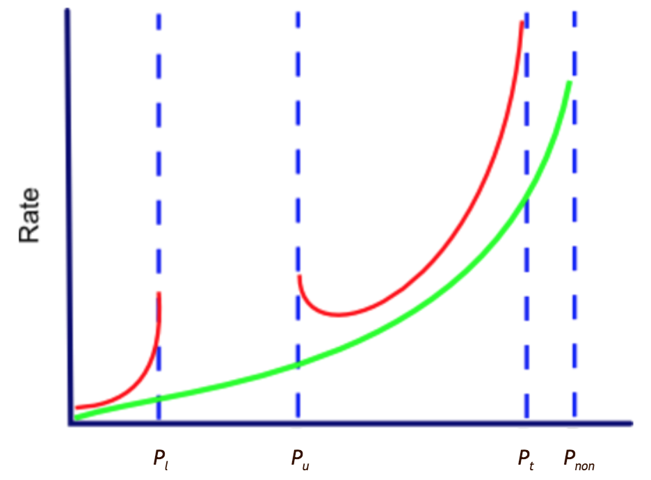
At a very low pressure range, the reaction is stable and occurs slowly. When the pressure reaches Pl (which is the first or lower limit pressure), the reaction becomes extremely fast (i.e., explosive). As the pressure increases further, the reaction is explosive until Pu (which is the second or upper limit pressure) is reached. Above this pressure, the reaction again reaches steady state, and no explosion occurs. The reaction is steady state until Pt (which is the third limit pressure) is reached, and the reaction becomes explosive again. These pressure borders can be plotted as the function of pressure versus temperature. This plot is called "the explosion diagram" and is shown for a stoichiometric mixture of oxygen and hydrogen in a KCl-coated container in Figure 2.

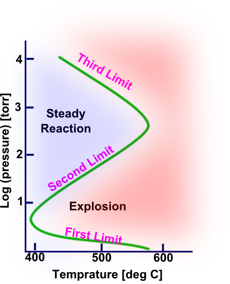
In the explosion limit diagram, the area to the left of the line represents the non-explosive reaction region and the area to the right of the line is the explosive region. The area between the lower and upper limits is referred to as the explosion peninsula. The lower limit decreases slowly as the temperature is raised and it is also very sensitive to the nature of the surface. The upper limit can be increased or decreased depending on the inert gas. The third limit decreases rapidly with increasing temperature and is lowered by adding inert gases and by increasing the diameter of the vessel.

Theory

Reaction between Hydrogen and Oxygen

The chain-branching explosion reaction between hydrogen and oxygen has been studied thoroughly in the past several decades. The chemical equation of the reaction looks rather simple (equation 19). Actually, the reaction mechanism involves more than 50 elementary reactions. In order to understand the main features of the process, we will limit ourselves to the five following reactions:

Reactions (20) and (21) are the reactions of branching, since in these reactions one free radical produces three free radicals. Thus, the number of free radicals increases as a result of these reactions. Since reaction (20) has a higher activation energy than reaction (21), the rate of this reaction is slower, and it is usually the rate determining step in the process. Reaction (22) is the reaction of the chain propagation, since it does not change the number of free radicals. In reactions (23) and (24) the number of free radicals decreases, and these reactions are called chain termination or chain breaking reactions. Although reaction (24) looks like a chain propagation reaction, the radical HO₂ is a rather inactive radical, and therefore it decays more rapidly on the wall than it reacts with other molecules in the gas phase. Thus, for simplicity, the reaction (24) can be considered as the termination reaction and HO₂ can be considered as a final product of the total reaction. In reaction (23), the wall is the inert container. In reaction (24), M is an inert molecule that the absorbs excess kinetic energy due to the reaction as will be explained further below.

Chain-Branching Reaction Kinetics

In a mixture of hydrogen and oxygen, it is plausible that the presence of a free radical in the form of OH radical or an H radical initiate reactions (20) to (21) to (22). The first reaction (H⋅+O2) is endothermic by 17 kcal/mol. Thus, at room temperature and even at somewhat higher temperatures a mixture of hydrogen and oxygen is very stable. The free radical generally reacts with the wall through a recombination process and terminates the reaction. At a critical temperature, however, the chain-branch reaction becomes sufficiently frequent relative to the rate of removal of H radicals by reaction with the wall to cause multiplication of free radicals and an explosion.

Explosions are conveniently classified into two distinct categories: branched-chain explosions, in which the reaction rate increases without limit because of chain branching, and thermal explosions, in which there is an exponential increase in reaction rate resulting from exothermic chemical reaction, heating of reactants, and an increase in the magnitude of the specific reaction rate constants.

Consider a 1 cm³ container that initially contains one chain molecule, that is, there is one free radical per centimeter cube. Assume that the number density in the container is 10¹⁹ molecules per cm³ (close to 0.5 atm at normal conditions) and the average collision rate is 10⁸ collisions per second. If the reaction in the volume is a chain-propagation reaction in which one free radical can generate another free radical (α, the coefficient that represents the mean number of free radicals produced in one reaction cycle, is equal to 1.0), then the time required for all of the molecules to react (i.e., 10¹⁹ collisions) will be:

Such a slow process cannot be called combustion. If the reaction is a chain-branching reaction, one free radical or chain particle can generate two chain particles (α = 2.0), and the time required for all of the molecules to react can be estimated as follows: The process in which every radical generates two additional radicals generates the following number of radicals:

Given that N = 62 generations solves this equation and that the average collision rate is 10⁸ collisions per second, one can calculate that all the molecules will react in 62·10^-8 seconds (~ 1 µs). This is certainly an extremely rapid combustion process. In an actual combustion process, not all reactions are chain-branching reactions. However, the reaction rate can still be very fast even if a small portion of the total reactions are chain-branching reactions. The coefficient α can, in this case, be closer to 1 than 2.

Exercise: calculate the time required for all molecules in the volume to react in a combustion process in which just 1% (α=1.01) of the elementary reactions are of the chain-branching type.

Surface Termination Reactions

Chain termination, which occurs as a result of the interaction of free radicals with the walls of the reaction cell, plays a very important role in many gas-phase chain reactions, especially at low pressures. Destruction of radicals on the wall is a result of two consecutive processes: diffusion of the radicals to the wall and the interaction of the radical with the surface. If the first process is the rate-limiting step (diffusion is slower), the reaction is said to take place in the diffusion region. If the interaction with the wall is limiting, the reaction is said to takes place in the kinetic region. Effectively, the reaction occurs as a first-order reaction with rate constant k:

where $κ_d$ is called the diffusion rate constant, which, for the cell with characteristic size d, is equal to:

This reaction can be easily understood when compared with the Einstein diffusion equation $<\Delta x^2>=2NDt$ (for N dimensions). The coefficient A depends on the shape of the cell; for example, A=39.6 for a sphere, and A=23.3 for a very long cylinder. In a gas, diffusion rates are determined by collisions between the molecules, and their average speed. The diffusion coefficient D depends on temperature and pressure as follows:

where $D_0$ is the diffusion coefficient under normal conditions, $T_0$ and $P_0$. Thus, the rate constant κ_d is:

The rate constant of the reaction on the surface can be calculated based on the gas kinetic theory:

where ε is the chain termination efficiency of the radical collision with the wall, v is mean radical velocity, S is the cross section of the radical collision with the wall, and V is the volume of the cell. The coefficient ε strongly depends on the quality and the type of the wall surface as well as on the type of the radical. Usually $ε is approximately 10^{-5}-10^{-2}$ for glass and quartz and $ε approximately 10^{-2}-10^0$ for metals.

Gas-Phase Recombination Reaction

The gas phase recombination reaction (24) is sometimes called a termolecular reaction. In the case of the reaction of hydrogen and oxygen, the reaction is not truly elementary one, but composed of two consecutive bimolecular steps. Therefore, to be accurate this reaction should be referred to as a third-order reaction since the term termolecular can only be applied to a reaction involving simultaneous collision of three species. Let us consider the reaction of two atoms A and B, which forms a molecule AB in the presence of a third molecule M:

The "third body" molecule, M, is needed since in the first elementary step with a rate constant $k_a$ is:

the molecule $AB^{\star}$ is a "hot" molecule, which has energy equal to the formed bond energy plus the kinetic energy of the atoms. Therefore without the third molecule body M, the molecule $AB^{\star}$ will dissociate very rapidly, with a rate constant $k_b$, during one molecular vibration:

The third body M can absorb excess of the energy from AB^★ and convert it to the stable molecule AB, with a rate constant $k_c$:

Applying the steady-state hypothesis to the excited molecule AB^★, which is short lived and is present in a very small concentration we obtain:

Therefore in the steady state:

The rate of product formation is:

In case of atoms or small radicals the lifetime of $AB^{\star}$ is very short, meaning that the rate constant k_b is high. Therefore at of less than 1 atm $k_b≫k_c·M$, and the approximate rate of product formation (from equation 2) is:

Thus, if we consider this reaction as a reaction of third order between A, B, and M, the third-order rate constant is equal to $κ^{(3)} = κ_a·κ_c/κ_b$. The units of this constant are $cm^6/(mol^2·sec)$.

Alternatively, we can consider the bimolecular reaction A + B → AB, which has a rate constant that depends linearly on the concentration of M: $κ^{(2)} = (κ_a·κ_c/κ_b)·M$. In this case the units are $cm^3/(mole·s)$. As a more complex radical than $M^{\star}$, the lifetime of the excited molecule $AB^{\star}$ is longer than that of $M^{\star}$ since the excess of energy can be redistributed to the different internal degrees of freedom. Thus, even at atmospheric pressure, $κ_b≪κ_c·M$, and the reaction can be considered second order with rate constant $κ_∞=κ_a$.

Let us consider in more detail the first case of the third-order reaction. In this case energy is transferred from the molecule $AB^{\star}$ to the vibrational or rotational energy of the molecule M. The rate constant of the deactivation or relaxation, $κ_c$, strongly depends on the type of the deactivator, M, and is related to its ability to absorb the excess energy. First the rate constant is higher for light molecules than for heavy molecules, since lighter molecules can more readily convert absorbed energy to kinetic energy. Second, it is higher for molecules with more degrees of freedom than for those with few degrees of freedom. Usually, the total rate constant of the reaction decreases as temperature increases. This can be explained in the following way: The rate constant $κ_a$ does not depend significantly on temperature, since it has no or minimal energy of activation. In contrast, the rate constant $κ_b$ increases with increasing temperature, since at higher temperatures the kinetic energy of atoms and molecules is higher and will increase the excess energy of the excited molecule AB* facilitating dissociation. The reaction of relaxation, with rate constant $κ_c$, also has no dependence on temperature. Thus, because of the growth of $κ_b$ with temperature, the total rate constant will decrease. It can be treated mathematically as the reaction with "negative" activation energy.

Solving the Kinetics Problem with Ordinary Differential Equations

In order to solve the kinetics problem, we need to build a system of coupled differential equations using the appropriate rate constants $κ_1-κ_5$, for the reactions of equations (20 - 24) as well as the rate of radical initiation, $ω_i$:

This is a system of nonlinear differential equations that cannot be solved analytically. During the computer experiment you will solve it numerically. In the framework of the so-called quasi-steady-state approximation, this system can be treated analytically. Within the limits of this approximation we will consider only the first three equations, since we will be interested in the early moments of the explosion when the change in hydrogen and oxygen concentration is insignificant. Since the concentration of O and OH are usually much lower than that of H, in the early moments of the explosion, $(d[O]/dt)=(d[OH]/dt)=0$. Therefore:

or

where the branching factor φ is the difference between the rate of the branching reactions and the rate of the termination reactions:

In case of constant φ (neglecting the change in concentration of oxygen) the solution of the equation (45) is:

The system behavior falls into two clear-cut cases depending on whether the branching factor φ is greater than or less than zero. When φ<0 the reaction shows "normal" behavior approaching steady state (Figure 3, blue line). When φ>0 the variation of rate with time follows a continuously accelerating, exponential, rise as shown in Figure 3 (red line). The sharp division between these two types of behavior is expressed by the condition φ = 0.

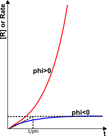
The plot in Figure 3 shows that there is an explosion limit at which a very small change in conditions, such as the temperature, pressure or composition of the reactants, can change the reaction rate from a slow steady value to one that is self-accelerating and that will eventually become infinitely fast. When the rate of reaction reaches a certain value the observable characteristics of an explosion appear such as a shock wave (causing a bang to be heard) and high temperature (causing a flash of light to be seen). There is, however, a time-lag before the rate reaches this critical value: That is, there is an induction period before explosion. This may be of the order of milliseconds or minutes depending on the value of φ.

Let $[H]_{crit}$ be the critical active hydrogen center concentration at which the rate is just fast enough to produce an explosion. Then if $t_i$ is the induction period:

The logarithmic term in this equation varies relatively slowly with φ so we can make the approximation that: $t_i$ is approximately equal to $1/φ$.

This result shows that large net branching factors result in short induction periods before explosion while small net branching factors, only very slightly in excess of zero, lead to very long induction periods. Although this discussion of explosion limits has been restricted to linearly branched and terminated chains for simplicity, it nevertheless enables us to interpret the experimental data of a number of branched chain reactions.

Thus, first and second explosion limits can be found from setting the condition φ = 0 in equation (46):

The concentrations depend on pressure and temperature. According to the ideal gas equation, the concentration of a molecule is proportional to its parial pressure by:

where $\chi_i$ is the mole fraction of the specie i.

We will assume that the diffusion to the wall is the rate determining step for the wall termination. We can therefore substitute equations (26), (28) and (50) in equation (49), and find:.

where

This is a cubic equation for P and as can be seen from the signs of the terms, two of the roots are positive and one is negative. The latter cannot correspond to any physically observable system but the two positive roots account for the lower and upper explosion limits that are observed.

At the lower limit $P_l$, the principal termination reaction is the surface, the gas-phase termination is small so that we have approximately:

and

At the upper limit $P_u$, gas-phase termination is more important than surface termination so that equation (51) becomes approximately:

or

We can replace the rate constants in equations (54) and (56) with the Arrhenius equation to derive the relationship between the upper and lower pressure limits and the activation energies.