Explosion - A Reaction between Oxygen and Hydrogen
In this experiment you will study the kinetics of explosion reactions using a simulator.
Experimental procedure
Part One
Numerical Simulation of First-Order Reaction
We will start by simulating the following simple first-order reaction:
$C_2H_6 (g) \rightarrow 2CH_3 (g)$
The reaction's rate constant is $k=5.36·10^{-4} [s^{-1}]$ at a temperature of 700 °C.
- Using equations (17) and (18), calculate and plot the reactant concentration vs. time between $t_i=0 [s]$ and $t_f=20,000 [s]$. Assume reactant concentration of 1 [M] at time $t_i=0 [s]$. You can find an illustrated guide for an Excel simulation here. Working on other platforms, such as Matlab or Origin, is possible as well.
- Compare the numerical results with the analytical solution (equation (16)).
- Plot the reactant concentration vs. time for five different time steps, $\Delta t$, in the range from 50 to 3,500 [s]. You will have five different graphs. What happens in each limit? When does the numerical solution approach the analytical solution and why?
- The activation energy of the reaction is $E_a=385 [\frac{kJ}{mol}]$. Use the Arrhenius equation to calculate the rate constant at temperatures of 600 °C and of 800 °C .
- Run the simulation again for each rate constant (that is, for each temperature). If necessary, change the time step and/or the simulation length. What happenes when you change k? Why did you have to change $\Delta t$?
Numerical Simulation of Complex Reaction
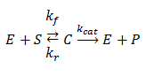
Enzymes are catalysts that increase the speed of a chemical reaction without themselves undergoing any permanent chemical change. One of the simplest models to describe enzyme activity is the Michaelis-Menten model. According to this model, a substrate S binds reversibly to an enzyme E to form an enzyme-substrate complex C, which then reacts irreversibly to generate a product P and to regenerate the free enzyme E. This system can be represented schematically as follows:
Such a mechanism cannot be solved analytically without approximations. Here we will solve it numerically.
- Write down the rate laws for all of the reaction components (E, S, C, and P).
- Using Euler's method, derive the set of recurrent equations that you will calculate in your simulation.
- Solve the equations numerically using your chosen platform (Excel, Matlab, Origin) between $t_i=0 [s]$ to $t_f=500 [s]$. Use the following conditions: $E_0=20 [mM], S_0=50 [mM], C_0=P_0=0 [mM], k_f=0.001 [\frac{1}{mM·s}], k_r=0.0001 [1s], k_{cat}=0.1 [\frac{1}{mM·s}]$.Choose a time step, $\Delta t$, that enables a good resolution.
- Plot the concentration of E, S, C, and P vs. time on the same graph. How do concentrations of these components change during the reaction?
- Plot the concentrations of the components at five different initial concentrations of the enzyme and of the substrate between 10-100 mM with the ratio fixed at 1:1 (you will have five different graphs). If necessary, change the time step and/or the simulation length. How does concentration influence the reaction?
- Under certain conditions, a quasi-steady-state occurs, in which the complex concentration C is approximately constant during the reaction. Find conditions (that is, $E_0$ and $S_0$) under which this quasi-steady-state is established, and conditions under which it does not occur. You will need to change the ratio between the concentrations of $E_0$ and $S_0$ from 1:10 to 10:1. Again, if necessary, change the time step and/or the simulation length. Show the plots and explain your findings.
Part Two
Find the Explosion Peninsula in a Stoichiometric Ratio
- Set your system temperature to 800 °K and find the lower and upper explosion limits at this temperature. Think very carefully: How should you determine these boundaries? What was the maximum time that you used? How did you determine it?
- Plot ln(P) versus the temperature. Fill out the table below. Compare your result to Figure 2.
A remark: You may run into trouble finding the lower and upper limits at the temperature of 800 °K. If that happens, search the lower and upper limits at 820 °K instead.
| T °K | P [Atm] | ln(P) [Atm] | |
|---|---|---|---|
| Lower Limit | 800 | ||
| 840 | |||
| 860 | |||
| 900 | |||
| 940 | |||
| 980 | |||
| 1020 | |||
| Upper Limit | 800 | ||
| 840 | |||
| 860 | |||
| 900 | |||
| 940 | |||
| 980 | |||
| 1020 | |||
Find the Activation Energy for the Branching Stage and the Termination Stage
Stage
Use the data obtained in the previous section to calculate the activation energies of the branching reaction and the termination reaction. Fill out the table below (make sure that you use the correct physical units):
| Calculated Energy | Literature Value | |
|---|---|---|
| Branching | ||
| Termination |
Discuss your results.
Validate that the Steady-State Assumption is Valid for [O·] and [OH·] in the Explosion Region
1. From the analysis of the explosion peninsula in the first exercise, select a point ($T_1$, ln($P_1$)) in the explosion limit. Run the simulation and extract the concentrations of radicals H·, O·, and OH· and of the reactants H2 and O2 versus time.
Note: You do not enter a time interval for the simulation. The algorithm sets the time interval by it self!
This is the table you should fill out (more rows are needed):
| time | Concentration of: | ||||
| H· | O· | OH· | H2 | O2 | |
| ... | ... | ... | ... | ... | ... |
- Plot a graph of the radical concentrations versus time and the reactant concentrations versus time.
- Is the assumption of steady state valid?
- What was the maximum time that you used?
- How did you determine it?
Calculate the Net Branching Factor, φ, for Two Different Pressures at the Same Temperature in the Explosion Region
- Select two points from the explosion peninsula graph from the first exercise, ($T_1$, ln($P_1$)) and ($T_1$, ln($P_2$)), that are in the explosion limit (make sure that you pick the same temperature). Calculate the branching factor, φ, of the two points (use equation (47)); note the time interval you use for this calculation. Before moving to the next part of the experiment try to draw a qualtitaive plot of φ as function of the pressure. Remember that in the limits of the explosion peninsula φ > 0
- One point has a larger branching factor than the other. Why?
Evaluate the Effect of the Stoichiometric Ratio of the Reactants $H_2$, $O_2$
- Evaluate the explosion peninsula graph at stoichiometric ratios of the reactants $H_2$ and $O_2$ of 3:1 and 1:1 and compare these graphs to the explosion peninsula from the first exercise, when you worked with stoichiometric ratio 2:1. Fill out the table below (more rows are needed):
- Plot the three peninsulas on the same graph and discuss the changes in the explosion boundaries. Explain your observations.
| Limit | temperature | $H_2$, $O_2$ (2:1) | $H_2$, $O_2$ (1:1) | $H_2$, $O_2$ (3:1) | |||
| Lower | ... | ... | ... | ... | ... | ... | ... |
| ... | ... | ... | ... | ... | ... | ... | |
| ... | ... | ... | ... | ... | ... | ... | |
| Upper | ... | ... | ... | ... | ... | ... | ... |
| ... | ... | ... | ... | ... | ... | ... | |
| ... | ... | ... | ... | ... | ... | ... | |
Add Water Vapors and Inert Gas (N2) to the Initial Conditions
- Add 1/31 of water to the initial conditions while keeping the ratio between $H_2$ and $O_2$ at 2:1. Compare this explosion peninsula graph to the graph from the first exercise.
- Add 4/7 inert gas ($N_2$) to the initial conditions while keeping the ratio of $H_2$ to $O_2$ (2:1). Compare the explosion peninsula graph to the graph from the first exercise.
- Fill out the table below (more rows are needed):
| Limit | temperature | $H_2$, $O_2$ | $H_2$, $O_2$, $H_2O$ Calculate the correct ratios |
$H_2$, $O_2$, $N_2$ Calculate the correct ratios |
|||
| Lower | ... | ... | ... | ... | ... | ... | ... |
| ... | ... | ... | ... | ... | ... | ... | |
| ... | ... | ... | ... | ... | ... | ... | |
| Upper | ... | ... | ... | ... | ... | ... | ... |
| ... | ... | ... | ... | ... | ... | ... | |
| ... | ... | ... | ... | ... | ... | ... | |