SEE Workshop Tutorial
Introduction
SEE-workshop is the basic stand-alone version of SEE. Since it's the basic version of the software, it will be referred to in this tutorial simply as " SEE“.
This tutorial was written for quick but thorough learning of SEE. It contains practical information as well as explanations of concepts and methods used in the software. Following it, you should be able to produce high quality data – a basic requirement for replicable studies.
Lessons 3 to 7 provide information on the methods used in each module of SEE as well as instructions to run the analysis step by step and proper setting of parameters.
Lesson 9 is a practical summary of these lessons. It provides the full analysis protocol without the theoretical information.
For more information on SEE, check out the overview and publications.
Lesson 1 – Download, installation and file preparation
SEE download and installation
To install SEE:
- Click DOWNLOAD
- Unpack SEEsetup.rar.
- Run SEEsetup.exe.
- Follow the instructions in the setup window.
To run SEE, double click on Workshop.exe in the installation folder.
Preparing a folder system
For this tutorial, create the following folder and subfolder: C:\tutorial_01
To best use SEE, each tracking file should be placed in separate folders.
SEE produces 13 output data files that are saved in the same folder as the input tracking file. Therefore, to avoid confusion it is recommended to put each file in a separate subfolder of the main experiment directory.
Preparing a tracking file for analysis
SEE analyzes raw XY tracking coordinates of a single animal. Different tracking programs produce coordinates in different file formats (*.txt, *.csv, *.xlsx etc.).
SEE requires a CSV (comma delimited) file.
Tracking with Noldus Ethovision XT
Older versions of Noldus Ethovision export raw data into a CSV file. However, in newer versions the data is exported into Microsoft Office *.xlsx files. In that case, simply open the file and save it as CSV.
Note: the trial description lines at the top of the table are OK to keep while converting to CSV.
Tracking with other programs
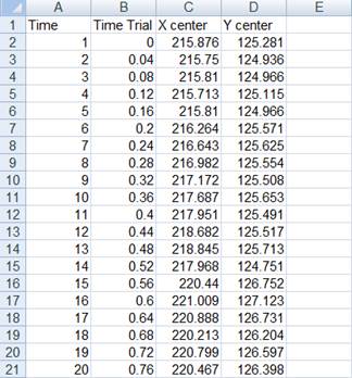
According to the tracking software you use, your file may require rearranging in order for SEE to read it. The file should be arranged in 4 columns in the following order:
- Time – frame number (a running index from 1 to the last frame of tracking)
- Time trial – the time stamp in seconds of each coordinates, according to tracking sampling rate* (25 Hz – 0.00, 0.04, 0.08,… 30 Hz – 0.033, 0.067, 0.010,…)
- X center ** – X coordinate
- Y center ** – Y coordinate
*Note – the tracking sampling rate may differ from the filming sampling rate, especially in real-time tracking. For example – filming may be 25 Hz and tracking 5 Hz.
**Note – the XY coordinates should be the raw data, before smoothing. If your tracking software features path smoothing, disable it before exporting the data.
This is an example of a tracking CSV file, tracked at 25 Hz:
Now take one of your tracking files, rearrange it if necessary, and save it as file_01.csv in the folder C:tutorial/file_01.
When you finish all preparations, open SEE and proceed to lesson 2.
Lesson 2 – Main screen
This lesson provides an overview of the main screen's functions.
The progress of the analysis in this tutorial is limited to adding your tracking file to SEE. Performing proper analysis depends on setting the right parameters, and therefore we shall perform segmented analysis over the next lessons.
Main screen
The main screen of SEE is where you select a tracking file and run the analysis.

Selecting a file for analysis
Continuing from lesson 1 , you should have a CSV file containing tracking coordinates with the full name C:\tutorial_01_01.csv.
In SEE main screen, in the Folders section, press Add…

Now choose your file path in the left panel. If you chose the correct path, the name of your file should appear on the right.
Press OK to finish. The Folder section will now contain your file's path.
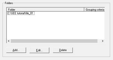
To edit a path, select it an press Edit. To delete, select the path and press Delete.
Note: it is recommended to add only one path at a time. In case of two or more the analysis will only be performed on the top one.
Selecting SEE modules
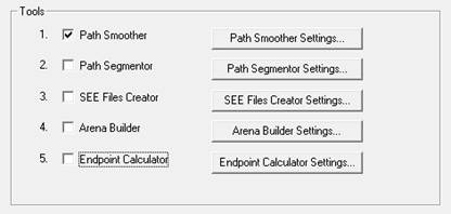
In the Tools section you can select which SEE module to run and open the settings window of each one.
There are five modules:
- Path smoother - lesson 3
- Path segmentor - lesson 4
- SEE files creator - lesson 5
- Arena builder - lesson 6
- Endpoint calculator - lesson 7.
The following lessons will explain the input parameters require to run each module properly.
To select a module, check the checkbox next to its name. Check all checkboxes to run complete analysis.
To open the settings window, press the Settings button with the relevant name.
In this example, the Path smoother is selected:
Note: Each of the SEE modules can run separately in the Tools section. However, each module requires the previous module's output, so they should run in order.
Running analysis
To run analysis on the selected modules, press the Process button at the bottom.

Visualization of Smoothing will be explained in lesson 3.
At the end of this lesson, the path of yourtracking file C:tutorial_01 should be in the folders table. Proceed to lesson 3.
Lesson 3 – Path Smoother
SEE Path Smoother has three objectives:
- Smoothing the XY coordinates (with LOWESS)
- Calculating momentary velocities and accelerations
- Finding stops in the animal's movement (“arrests”) by smoothing the XY coordinates with Repeated Running Medians (RRM).
This lesson should help understanding how to use the Path Smoother module properly, and the theory behind it.
To skip the theory and the settings, just jump straight to Running Path Smoother (but don't cry if your analysis is bad).
Path Smoother settings
In the main screen (lesson 2), press Path Smoother Settings…
The following sections are both practical and theoretical and provide useful information required to produce better results using the Path Smoother.
Path smoother settings are divided to general settings, selecting a smoothing method for the animal path and selecting a method to define arrests.
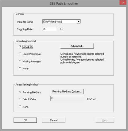
General
Smoothing Method
SEE suggests 4 possible methods to smooth the animal XY coordinates:
- LOWESS (recommended)
- Local Polynomials
- Moving Averages
- None
Select LOWESS and press Advanced… to set the smoothing parameters.
Why LOWESS?
Due to the animal's body wobble and the video resolution, a tracking software calculating the pixel containing the animal's geometrical center may produce different results in two consecutive frames, even though the animal was stationary.
As the velocity is the derivative of position, and the acceleration is the derivative of velocity, the noise in position results in very high momentary velocities and much higher momentary acceleration.
Therefore, None is not recommended and a smoothing method should be applied. The next example (Hen et al, 2004) shows the LOWESS advantages over the two other methods suggested:
- Moving Averages - smoothes the noise but also pushes curves towards their center, and so shifts the animal's position from its actual coordinates. In addition, it does not handle outliers well (e.g the tracking software had lost the animal for a few frames and identified a distant object instead, causing a sharp jump in position).
- Local Polynomials - better captures the curvature of the path and enables calculating velocities and accelerations as derivatives of the fitted polynomials, but has a similar problem with outliers.
- LOWESS - has the advantages of Local Polynomials but also eliminates outliers, making it the best option for path smoothing.
Advanced… (setting LOWESS parameters)
Most LOWESS defaults should not be changed unless you have the required knowledge in this method of smoothing.
Half a Window Width of 0.4 seconds (default) should work fine for most sampling rates. Increasing it will result in stronger smoothing.
In sampling rates of 5 Hz or lower it is recommended to increase the Half a Window Width value to 1 second.
This is an example of a path of mouse, smoothed with LOWESS using the default parameters:
Arrest setting method
Arrests may be found using Running Medians or by a certain cut-off value. No arrests means no progression/lingering segmentation.
Select Running Medians and press Running Medians Options… to set the parameters.
Note: setting the Running Medians parameters is crucial for segmentation (lesson 4). It is highly recommended to follow the instructions in the sections What are arrests? and Running Medians Options….
What are arrests?
As explained in the section Why LOWESS? the center of a stationary animal may shift during tracking. In order to analyze movement segments (lesson 4), we first need to isolate these non-movement segments (“arrests”).
LOWESS overcomes outliers and provides a good smoothed path, but it does not isolate time segments with minimal shift in position. For that we use Running Medians (RM).
RM is similar to Moving Average, but uses the median of each window instead of the mean, which shifts with the change of a single point (moving window). The results is, rather than a smoothed set, a rough segmented set where close coordinates are pushed towards a single point and therefore can be isolated as arrests.
Let us consider the parameters Set Arrests As and Cut Off Value in Running Medians options - a single arrest is a time period equal to or greater than the value of Set Arrests As, in which the distance between the two farthest coordinates of the animal (after RM) is less than the Cut Off Value.
In practice, a larger Cut Off Value will result in longer and more frequent arrests, and a larger Set Arrests As value will filter short arrests.
Running Medians Options…
Setting the RM parameters is crucial for the segmentation (lesson 4) to be performed properly:
- Sequence – a sequence of window widths for repeated RM. The sequence 7,5,3,3,0,0,0,0 has proved effective for all types of paths.
- Set Arrests As – should typically be 5 frames(default) for sampling rate of 25 Hz, and 6 frames for 30 Hz. If your tracking sampling rate is 5 Hz or lower, set 2 or 3 frames.
- Cut Off Value - Depends on the size of the animal and the arena and the video resolution. Larger animals and lower video resolution require larger cut off value. Mice – 1e-006 cm (default) is usually enough. Rats - 0.01 to 1.5 cm
Running Path Smoother
If you followed the instructions in lesson 2, the path of your tracking file should appear at the top of the folders section of the main screen.
Perform the following steps to run the Path smoother:
- In the main screen, in tools , check only (for now) Path Smoother.
- Set the parameters in Path Smoother Settings… according to the instructions in this lesson.
- Press Process.
- When you get the DONE message, press Close.
Path smoother output files
The following output files should now be saved in the same folder as your CSV file:
- file_01.txt - smoothed coordinates, velocities and accelerations
- file_01.inf - general information. The file is updated as the analysis progresses.
For more information about the output files, see lesson 8.
Visualization of Smoothing
The Visualization of Smoothing button at the bottom of the main screen displays the raw and the LOWESS smoothed path for comparison. Press it.
In the Open window, open your CSV file.
The smoothed X coordinate will appear in blue and the raw data in red, within the time frame defined in the Frames section. You may switch to the Y coordinate and calculated momentary velocities as well.
To change the time frame, set From frame and To frame and press Update.
Lesson 4 – Path Segmentor
SEE Path Segmentor the motion segments, distinguished from arrests by the Path Smoother (lesson 3), into progression and lingering.
Note : The quality of the segmentation is affected directly by proper isolation of arrests. Therefore, if the Path Segmentor produces bad results, it is most likely due to not setting properly the Set Arrests As and especially Cut Off Value in Running Medians Options….
To skip the theory and the settings, just jump straight to Running Path Segmentor (but don't cry if your analysis is bad).
Path Segmentor Settings
In the main screen (lesson 2), press Path Segmentor Settings…
File Format and Automation
In Input File Format ,keep Lowess output (*.txt).
In Automation , it is recommended to select Let me review…
This option provides visualization of the segmentation to better assess its quality (explained later in this lesson). Choosing the Accept all thresholds automatically should be used when you analyzed a few tracking files and you are sure of the Smoother and Segmentor parameters.
Progression and lingering segments
A motion segment is defined as a time segment between two arrests. The Path Segmentor divides these segments into two groups – lingering , consisting of very slow movement or complete arrest, and progression , where the animal reaches high maximal speed.
The Path Segmentor calculates the maximal velocity per motion segment, and then applies the EM algorithm to fit 2 Gaussians to the frequency distribution (density) of these velocities after log transformation.
The intersection of the 2 Gaussians will be considered the maximal velocity threshold , and then:
- Progression - all motion segments with maximal velocity higher than the threshold.
- Lingering – all other segments, including arrests.
This is an example of segmentation of the movement of a single mouse (represented by momentary velocity per frame) in some time frame during the experiment:
This is an example of visualization of the maximal velocities density and the EM fit, viewed be selecting Let me review… in Automation :
Finding the correct maximal velocity threshold
A proper density plot should have two distinct peaks – low max velocities (lingering) and high max velocities (progression). If so, SEE will calculate the proper value.
The shape of the frequency distribution is affected directly by finding arrests. If the density plot is way off, run Path Smoother again with different Cut Off Value in Running Medians Options.
This in an example of setting the Cut Off Value too high.
In cases of three distinct peaks, there is an option to fit three Gaussians. See Density Visualization later in this lesson.
EM Options and Density Options
The EM and Density Options hold in most cases. The Log(2+x) transformation should be kept.
Running Path Segmentor
Continuing lesson 3 , there is already a smoothing data file saved as file_01.txt in the same folder as the tracking file.
Perform the following steps to run the Path Segmentor:
- In the main screen, in tools , check nly Path Segmentor.
- In Path Segmentor Settings… select Let me review…
- Press Process.
- The Density Visualization screen pops up (see next section). Press Accept*.
- When you get the DONE message, press Close.
*Note: assuming the segmentation is acceptable.
There are no output files for the Path Segmentor, but the maximal velocity threshold is added to file_01.inf.
Density Visualization Screen
The Density Visualization screen is a tool to assess the quality of segmentation, as explained in the Finding the correct maximal velocity threshold section.
Besides the density plot, the most important thing here is the Threshold Value :
- Transformation - Log(2+x)
- Non Transformed - the maximal velocity threshold in cm/s
- Transformed=Log(2+Non Transformed) - the Gaussian intersection.
Note: proper threshold for mice and rats is usually between 10 and 30 cm/s.
In case three Gaussians are needed, press Add one. Note that the Threshold will be the intersection between the left and middle Gaussians.
To set the threshold manually, click on a point on the density plot and press Set Threshold.
Lesson 5 - Files Creator
The Files Creator produces output files according to the Path Smoother and Segmentor results.
Files Creator Settings
In the main screen (lesson 2), press SEE Files Creator Settings…
There is nothing important to change here. Make sure Use entire session is selected.
Running Files Creator
Continuing lesson 4 , after smoothing and segmentation of file_01.csv.
Perform the following steps to run the Files Creator:
- In the main screen, in tools , check only SEE Files Creator.
- In SEE Files Creator Settings… select Use entire session.
- Press Process.
- When you get the DONE message, press Close.
Files Creator output files
In addition to file_01.txt and file_01.inf, the following output files should now be saved in the same folder as your CSV file:
- file_01.dat - smoothed XY coordinates with time frames
- file_01.seg - all motion segments (excluding arrest segments), divided into segments with higher and lower maximal velocities than the threshold.
- file_01.ssg - the entire session divided into lingering (including arrests) and progression segments.
- file_01.spd - the magnitude of the momentary velocity vector per frame.
For more information about the output files, see lesson 8.
Lesson 6 – Arena Builder
The Arena Builder has two major objectives:
- Calculating the boundaries of the arena according to the animal path
- Wall/center separation
This lesson should help understanding proper use of the Arena Builder and its output.
Note: Arena Builder is applicable for circular open field arenas. It will not produce sufficient results in square or rectangular arenas, plus mazes etc.
Arena Builder Settings
In the main screen (lesson 2), press Arena Builder Settings…
The arena builder settings are divided to three categories:
- Calculating arena center and boundaries - sections Arena Builder Method, Arena Properties, Lowess Parameters and Miscellaneous
- Floor/Wall segmentation - sections Segments and Miscellaneous
- General - section Automation.
Automation is similar to Path Segmentor Settings (lesson 4). Choosing the option Let me review… will view, upon running the module, the Arena Visualization screen to assess the quality of the Arena Builder results.
The following sections in this lesson will explain the important parameters to set for good results.
Calculating arena center and boundaries automatically
The center and boundaries of the arena may be calculated automatically according to the path of the animal, or manually according to user definitions.
It is recommended to keep the default settings of Lowess Parameters and Miscellaneous sections of the settings window.
Automatic Calculation
The Arena Builder algorithm estimates the arena boundaries, under two assumptions:
- The animal tends to travel along the wall.
- The shape of the arena is not a perfect circle.
The algorithm finds the center of the arena, divides the arena into sectors (parameter Number of sectors in Arena Properties , default of 360 sectors) and calculates the coordinate of the arena boundary per sector.
While Number of sectors=360 usually produce sufficient results, we found that Number of sectors=720 produce better results in many cases.
This is an example of Arena Builder output with 360 sectors (left) and 10 (right), on the same smoothed path:
To apply the algorithm:
- Boundaries - in Arena Builder Method , choose By Mouth Path.
- Center - in Arena Properties , choose Calculate arena center automatically.
Calculating the arena boundaries manually
The algorithm may produce bad results if the animal does not travel along the wall. In that case, it is possible to define the boundaries manually, use the following settings in Arena Builder:
- Boundaries - in Arena Builder Method either choose By specified mouse and select the TXT file of the smoothed coordinates in another test, or Round arena with specified radius and set a constant radius in cm from the center.
- Center - in Arena Properties choose Enter arena center manually and set the X and Y values of center in cm.
Wall/center separation
In Segments , choose Move segments only (default). Otherwise, the wall/center separation algorithm does not depend on user definitions.
After defining arena center and boundaries, the algorithm calculates radial distance from the wall per frame, as well as the radial velocity (velocity component in the radial direction).
It then finds a threshold of radial distance from the wall, to separate the animal's path into near-wall coordinates and center coordinates. The progression segments, found by Path Segmentor, are divided into two types:
- Incursions – progression segments in the center of arena (radial distance of the animal from the wall is larger than the threshold during the entire segment)
- Wallcursions – progression segments near the wall (radial distance of the animal from the wall is smaller than the threshold during the entire segment)
This is an example of a single progression segment, divided into incursions (orange) and wallcursions (blue):
Arena Builder parameter Add to radius adds a specified length in cm to the estimated radial distance during wall/center separation, to guarantee that remain positive. It is unnecessary to change it.
Running Arena Builder
Continuing lesson 5 , after running Path Smoother, Path Segmentor and Files Creator on file_01.csv.
Perform the following steps to run the Arena Builder:
- In the main screen, in tools , check only Arena Builder.
- In Arena Builder Settings… set automatic calculation of arena center and boundaries as explained in this lesson.
- Press Process.
- The Arena Visualization screen pops up (see next section). Press Accept.
- When you get the DONE message, press Close.
Arena Visualization Screen
The Arena Visualization screen views the results of the center and boundaries calculation before separating the wall from the center.
Press Accept to continue, or Change Settings to open the Arena Builder Settings screen and change certain parameters.
Note: the Arena Builder is for circular arenas. With some success it can also handle polygons with rounded corners. If this is your case try decreasing the Relative window size in Lowess Parameters.
Arena Builder output files
In addition to file_01.txt and file_01.inf, the following output files should now be saved in the same folder as your CSV file:
- file_01.inf - adds radial velocity and distance thresholds.
- file_01.arn - XY coordinates of the arena boundary radius per sector
- file_01.arena - XY coordinates of the center, and number of sectors
- file_01.cur - divides progression segments into incursions and wallcursions
- file_01.dist - radial distance of the animal from the wall per frame
- file_01.hed2 - heading of the animal per frame
- file_01.rad - radial velocity (towards the center) of the animal per frame
For more information about the output files, see lesson 8.
Lesson 7 – Endpoints Calculator
The Endpoints Calculator analyses the data from the four previous modules and provides a series of endpoints for statistical analysis.
Endpoints Calculator Settings
In the main screen (lesson 2), press Endpoints Calculator Settings…
There are four groups of settings:
- General Properties - set the same Sampling Rate as you set in the Path Smoother (lesson 3).
- Time slices - an option not yet applicable.
- Homebase Properties - set Determine homebase automatically to calculate the animal's home base from its path.
- Arena Properties - set Arena Center , Arena Radius and Wall/Center Threshold according to output files of the Arena Builder (see Lesson 8).
Running Endpoints Calculator
Continuing lesson 6 , after running Path Smoother, Path Segmentor, Files Creator and Arena Builder on file_01.csv.
Perform the following steps to run the Endpoints Calculator:
- In the main screen, in tools, check only Endpoints Calculator.
- In Endpoints Calculator Settings… set the proper Sampling Rate.
- Press Process.
- When you get the DONE message, press Close.
The CSV file endpoints.csv , containing a table of endpoints, has now been saved in file_01 folder, and the homebase location was added to file_01.inf.
This concludes your file's analysis. Lesson 8 explains the output files now saved with your tracking file, and Lesson 9 provides a general protocol for full analysis.
Lesson 8 – Output Files
Upon completing SEE analysis on file_01.csv , its folder should contain 13 files excluding the original tracking file.
Note: All files are simple text tables and can be opened with notepad or any other word processor.
| Name/Suffix | Origin | Description |
|---|---|---|
| .txt | Path Smoother | Smoothed path, momentary velocities and accelerations |
| .dat | Files Creator | Smoothed XY coordinates per frame |
| .seg | Files Creator | Motion segments |
| .ssg | Files Creator | Progressions and lingering segment |
| .spd | Files Creator | Momentary velocity vector magnitudes |
| .arn | Arena Builder | XY coordinates of arena boundaries |
| .arena | Arena Builder | XY coordinates of arena center |
| .cur | Arena Builder | Incursions and wallcursions |
| .dist | Arena Builder | Momentary distance from wall |
| .hed2 | Arena Builder | Momentary heading |
| .rad | Arena Builder | Momentary radial velocity |
| .inf | Path Smoother, Files Creator, Arena Builder, Endpoints Calculator | Max. velocity threshold (lingering and progression), Distance and velocity thresholds (wall/center segmentation) and homebase coordinates |
| endpoints.csv | Endpoints Calculator | A series of endpoints for statistical analysis |
Output files detailed description
This section provides detailed description on each file.
Some files contain a table with no headers. In that case the columns are described from left to right.
.txt
Contains smoothed XY coordinates and momentary velocities and accelerations.
| Column | Description |
|---|---|
| X(cm) | Smoothed X coordinate per frame |
| Vx(cm/sec) | Momentary velocities in the X axis.The first derivative of the polynomial fitted by LOWESS during smoothing of the X coordinates. |
| Ax(cm/sec^2) | Momentary accelerations in the X axis.The second derivative of the aforementioned polynomial. |
| Y(cm) | Smoothed Y coordinate per frame |
| Vy(cm/sec) | Momentary velocities in the Y axis. |
| Ay(cm/sec^2) | Momentary accelerations in the Y axis. |
.dat
Contains only the smoothed XY coordinates with the time in frames.
| Column | Description |
|---|---|
| Index | Current frame. Multiplication by sampling rate returns the time in seconds. |
| X | Smoothed X coordinate per frame. |
| Y | Smoothed Y coordinate per frame. |
Note: the X and Y values are identical in the .txt file.
.seg
Contains all motion segments (no arrests), divided into segments with maximal velocity higher and lower than the threshold found by the Path Segmentor.
| Column | Description |
|---|---|
| Start frame | Starting time of the segment, in frames |
| End frame | Ending time of the segment, in frames |
| Type | 0 - highest velocity during segment lower than the threshold 1 - highest velocity during segment higher than the threshold |
| Spatial spread | The distance in cm between the two most distant positions of the animal during the segment |
Note: arrests are found between two motion segments. In this example, there were two motion segments in frames 1 to 16 and 29 to 30, and so there was an arrest between frames 17 and 28.
.ssg
Contains the entire session divided to progression segments and lingering segments (including arrests).
| Column | Description |
|---|---|
| Start frame | Starting time of the segment, in frames |
| End frame | Ending time of the segment, in frames |
| Type | 0 - lingering segment 1 - progression segment |
| Spatial spread | The distance in cm between the two most distant positions of the animal during the segment |
Note: lingering segments (type=0) contain motion segments with maximal velocity lower that the threshold combined with arrests. Therefore all segments in this example of the .seg file fall under the same first lingering segment. Segments with type=1 are identical in the .seg and .ssg files.
.spd
Contains the magnitude of the momentary velocity vector per frame: V(t)=Vx(t)^2+Vy(t)^2
Note: velocity 0 is an arrest.
.arn
Contains the XY coordinates of the arena boundary per sector.
The number of rows in this table is equal to the number of sectors entered in Arena Builder Settings.
.arena
The relevant values in this file are the xcenter and ycenter , which are the coordinates of the center of the arena.
The table below that contains the distance of each sector's boundary from the center.
.cur
Contains all progression (type=1 in the .ssg file) segments divided to incursions and wallcursions.
| Column | Description |
|---|---|
| Start frame | Starting time of the segment, in frames |
| End frame | Ending time of the segment, in frames |
| Type | 2 - wallcursion (progression segment near wall) 3 - incursion (progression segment away from wall) |
| Zero column | A magnificent collection of zeros. No other number allowed |
.dist
Contains the radial distance of the animal from the wall per frame.
Note: considering a mouse's body pressed against the wall, the distance of its geometrical center to the wall is about 2 or 3 cm and not 0 cm.
.hed2
Contains the animal's heading per frame. The heading is the angle (in degrees) between the line connecting the current and the next position of the animal, and a line perpendicular to the radius.
In this example (Horev et al, 2007) the angle alpha is the heading, the large arch indicates the arena wall, the empty circle is the mouse and the full circle is the arena center:
Note: -1 indicates arrest.
.rad
Contains the animal's velocity in the radial direction per frame.
Note: positive value indicates movement towards the center , negative is towards the wall and zero is an arrests.
.inf
Contains information related to the smoothing, segmentation and arena building.
These are the important values:
| Name | Description |
|---|---|
| mouse_info | The headers of the columns in the tracking CSV file |
| smoother | The tracking sampling rate |
| em | threshold - the maximal velocity threshold between lingering and progression |
| wallsegmentor | RadDistanceThreshold - the wall/center threshold. |
| homebase | The XY coordinates of the animal's calculated home base |
endpoints.csv
Contains a series of endpoints for statistical analysis.
General terms:
- Activity - the accumulated sum of distance between two consecutive points
- Duration - the amount of time between two points.
| Endpoint | Description |
|---|---|
| DST | Distance traveled (cm) during the entire session |
| LMS | Lingering Mean Speed (cm/sec). Activity during lingering segments divided by their total duration |
| CNTRT | Total time spent away from wall , divided by the duration of the entire session |
| CNTRL | Total time spent away from wall during lingering, divided by the duration of the entire session |
| CNTRL2 | Total time spent away from wall during lingering, divided by the total duration of the lingering segments |
| NP | Number of progression segments |
| SPTL | Median spatial spread during lingering segments (cm) |
| LNGP | Median activity of progression segments (cm) |
| DL | Median duration of lingering segments (sec) |
| Q5DP | 5th quantile of duration of progression segments (sec) |
| Q95DP | 95th quantile of duration of progression segments (sec) |
| MDP | Median duration of progression segments (sec) |
| Q95PS | 95th quantile of maximal speed in progression segments (cm/sec) |
| PMXS | Median of maximal speed in progression segments (cm/sec) |
| LMXS | Median of maximal speed in lingering segments (cm/sec) |
| MSDR | Acceleration to max speed (cm/sec^2). Median of maximal speed dividedby the segment duration in progression segments |
| DART | Evaluated by log10(MSDR/LMS) |
| TRT | Median of the absolute turn rate * in progression segments (degrees/sec).
The absolute turn rate of one data point is calculated in the following way:
|
| TRAD | Median of radius of turns in progression segments (cm), which equal the momentary velocity divided by the absolute turn rate per point. |
| LMXHS | The amount of time until the animal reached a speed of Vmax/2, where Vmax denoted the 99th quantile of progression segments maximal speeds. |
| DVRS | Let n denote the number of lingering segments. For i=1,2,...,n let (xi,yi) denote the point which is the average of all data point in the i'th lingering segment. Let pi denote the proportion of the duration of the i'th lingering segment, relative to the total duration of all lingering segments. The diversity is the sum, over all i,j=1,2,...,n of the terms pi*pj*distance((xi,yi),(xj,yj)). |
| CNTRA | Total activity during incursions segments divided by the total activity during all lingering segments |
| CNTRR | Total activity during away from wall lingering divided by the total activity during all progression segments |
| TL | Duration of lingering segments divided by activity in the entire session |
| MXSPTL | Maximal spatial spread in all lingering segments (cm) |
| HBR | Total time spent in home base during lingering, divided by the total duration of lingering segments. |
| NLA | Number of lingering segments divided by DST (1/cm) |
| NEXC | Number of excursions - an excursion starts with a progression segment during which the animal exits the home base, and ends with a progression segment during which the animal entered the home base. |
| NLEXC | 10% trimmed mean of number of lingering segments during excursions |
| LPT | The maximal velocity threshold between progression and lingering |
| HBO | This endpoint is used to determine the home base automatically. The home base relative occupancy is calculated as follows:
|
| DSTDR | Total activity in the second half of the session divided by the total activity in the first half of the session |
| MCP | Median of curvature during all progression segments.
The curvature (by fixed distance interval) of one data point is calculated in the following way:
|
| MCW | Median of curvature during wallcursions. |
| MCC | Median of curvature during incursions. |
Lesson 9 – Running complete analysis
This lesson provides a protocol to run SEE analysis quickly:
File preparation
- Save your tracking files in separate folders.
- Edit your tracking file to have 4 columns - Time, Time trial, X center and Y center. Save it as CSV.
- Open SEE.
- In Folders , press Add and choose your tracking file's path.
- Check ALL five modules.
Path Smoother settings
- Open Path Smoother Settings.
- Enter correct Sampling rate.
- In Running Medians Options , enter Set Arrests As and Cut Off Value properly according to your experiment properties.
- Don't change other parameters unless absolutely necessary.
Path Segmentor settings
- Open Path Smoother Settings.
- In Automation , choose Let me review…
- Don't change other parameters unless absolutely necessary.
Files Creator settings
- Open SEE Files Creator Settings.
- In Session duration , choose Use entire session.
Arena Builder settings
- Open Arena Builder Settings.
- In Automation , choose Let me review…
- In Arena Properties , set Number of sectors
- Unless manual calculation of arena center and boundaries is required, in Arena Builder Method choose By mouse path, and in Arena Properties choose Calculate arena center automatically.
- Don't change other parameters unless absolutely necessary.
Endpoints Calculator settings
- Open Endpoints Calculator Settings.
- Enter correct Sampling rate.
- In Homebase Properties , set Determine homebase automatically.
Run Analysis
- Press Process.
- In Density Visualization , press Accept.
- In Arena Visualization , press Accept.
- Rejoice! Analysis is complete!
Summary
The SEE tutorial is now over. You should now have the knowledge to produce high quality data sets from your tracking files:
- Smoothed animal path - Path Smoother
- Segmentation of the animal's movement to progression and lingering - Path Segmentor
- Arena center and boundaries – Arena Builder
- Incursions, wallcursions and radial distance threshold - Arena Builder.
The next step is to build your own statistical analysis based on this data, according to the requirements of your research.
For examples of studies which used SEE, refer to the publications.
Supported by European Research Council under the uropean Community’s Seventh Framework Programme, ERC grant 294519 (PSARPS)