Inductive Regression

Contents |
[edit] Purpose of Web Page
This page deals with with the probem of learning from values that have a continuous range of values. In other words this page describes Regression Analysis but from an inductive viewpoint.
[edit] Summary
Inductive Inference gives a framework for predicting future events based on past history. However there are particular problems when dealing with Real Numbers. A real number has a zero probability of any particular value, and it requires an infinite amount of information to represent most real numbers (the Irrational Numbers).
You would never see a real number in the data history. The Real Numbers are inferred from approximations based on Rational Numbers.
Bayes theorem may be applied to continuous probability variables (Bayes' Theorem for Probability Distributions) to infer probability distributions for events based on past history. Unfortunately this theorem needs prior distributions.
As for Inductive Infereence Information Theory gives us a basis for chosing prior distributions.
The inclusion of the probabilities of the models is necessary to avoiding over-fitting.
[edit] Inductive Regression
Inductive Regression attempts to estimate the probability of continuous variables (Real Numbers) based on past history.
[edit] Bayes theorem for Continuous Variables
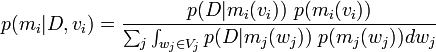
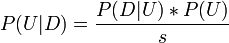
From Bayes' theorem alternate form,
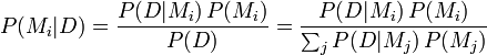 .
.
where j indexed over all models.
Now look at the case where the models are parameterised by constants. We may consider parameters that can be represented with a finite amount of data to be part of the code. However this approach breaks down when dealing with real numbers.
A real number is a very strange thing. Unless there is special way of representing the real number (e, Π, rational number, surd) a single real number has an infinite amount of information. Almost all real numbers have an infinite amount of information.
In order to deal with real numbers probability theory needs to be extended to use probability measures. A measure is a simple idea with a subtle twist. Length, Area, and Volume are all measures. The subtle thing is that a measure is a property of a set of points, that does not directly depend on the number of points in the set.
You will never see a real number in a data set. You will see only approximations. Normally an instrument will record a number to a certain number of digits. A real number is then an idea about the underlying universe that is inferred rather than seen directly.
[edit] Derivation of Bayes Law for Real Parameters
[edit] Reslicing the Pie
To deal with real numbers we will re-index the models so that the parameters to a model are used to identify the model,

where,
- K is the set of all models. Note that we have implicitly made this set uncountable.
- W is the set of parameterised models (with the real numbers removed and turned into parameters).
- Vi is a vector space of real numbers which parameterise mi.
[edit] Taking limits
Now we might like to plug our new list of models into the equation above but this is not possible. The probability P(D | mi(vi)) would be zero. The standard approach to take in this case is to divide the vector space up into areas of finite size, and consider the probability of the area. Then take the limit as the size d → 0.
A limit allows us to consider a number that is as small as we need it to be, but not zero. We can think of a limit as an approximation that we can make as accurate as we need.
[edit] Partition of Vector Space
In a small region the probability is the probability density function times the size of the region. To proceed we need to divide each vector space Vi up into equal sized pieces (lengths, squares, cubes etcetera, according to the dimension of the vector space). The dimension of the vectors space is the number of real parameters to the model mi. Dividing the vector space up in this way is a Partition of the vector space.
For simplicity here we will assume the existence of the probability density function and that it has an integral. A more rigorous proof would examine these issues.
Each of the equal sized pieces of Vi is named Ri(ni). The pieces are numbered by the vector of integers ni where  and Ni is a vector space of integers.
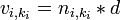
We can define the partition by a condition on each dimension of the vector. For each dimension ki in Dimensions(Vi),

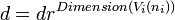
the size of Ri(ni) is,
[edit] Probability Density Function
Firstly let,

This multication of a vector by a scalar and means the sames as for 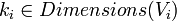 ,
,
The probability density function p is then,

The probability function p is the amount of probability per unit of the vector space.
[edit] Putting it all Together

or,

but,

[edit] Bayes' Law for Real Parameters
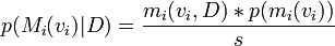
Putting the results together we have,
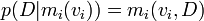
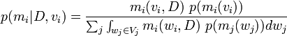
We use mi(vi) in two ways,
- As an event which identifies a set of outcomes.
- As a function that gives the probability of D given the model mi(vi).
The second use gives,
[edit] A-Priori distributions for the model
What then is p(mi(vi)). We can break this down as the probability of the model, times the probability of the value vi. The probability is related to the message length. To communicate the model, we need describe the model and then its parameters.
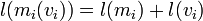
so,
We might want to use a uniform distribution for p(v_i). However this does not work. A uniform distribution is zero everywhere, and because of the sum over different models (with different numbers of parameters), the limits to zero cant be made to cancel out.
This problem needs further investigation.
[edit] Predictive Models
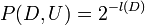
Some models of the data have a higher probability than the data,
These are the models that provide information about the behaviour of D. They are predictive models.
Other models are unpredictive models. Rather than deal with each unpredictive model separately we want to group them together and handle them all as the set U. Two sets of indexes J and K are created for the good and bad models,
is the set of indexes of models that are predictive.

is the set of indexes of models that are not predictive.
U as the union of the model events for which no data compression happens on the data history D.
Then we need to know,
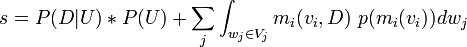
Bayes law with all the models that do not compress the data merged together becomes,
where
[edit] Real Numbers for Data
As stated before we will never see real numbers in the data set. However we will see approximations to real data.