1. TITRIMETRIC METHODS OF ANALYSIS

Titrimetric analysis consists in determining the number of moles of reagent (titrant), required to react quantitatively with the substance being determined. The titrant can be added (a) volumetrically, with a glass or automatic burette or with a low flow-rate pump, or (b) coulometrically, with an electrochemical generation from a proper electrolyte.

Titrimetric methods of analysis have the virtue of being like gravimetric methods, absolute in that the concentration of the substance in question is determined from the basic principles of chemistry, and no calibration curves are required.

Various methods are available for end-point determination: spectrophotometry, potentiometry, amperometry, conductometry, etc. The potentiometric end-point determination is the most widely used.

1.1. Modes of titration

Titrations are performed manually point by point, or automatically, where the titrant is introduced continuously (monotonically or dynamically). In modern analytical chemistry automation is of increasing importance. Automation of a point-by-point titration is seldom trivial. Kinetic factors concerning the chemical reaction and the response of the indicating system are of paramount importance. Cell configuration, stirring, positioning of end-point detector and of input of titrant are to be considered for ensuring high accuracy.

Equilibrium throughout the titration curve can be attained only when the titrant is added at an infinitely low rate. Two factors determine the rate at which a potentiometric curve approaches the state of equilibrium: the kinetics of the chemical reaction and the kinetics of the electrode process. Both factors are slowest in the vicinity of the equivalent point (why?), the region with utmost importance, from which the end point is determined (Fig.1-1a). (In conductometric titrations, on the contrary, the region around the end point is of no analytical importance; the end point is determined by extrapolation from the left and right branches of the titration curve away of the end point). At faster titration rates compared to the kinetics of the system, a delayed end point is obtained (Fig.1-1b).

Fig.1-1 Continuous potentiometric titrations

The degree of the delay of the end point depends on the concentration of analyte, the composition of the solution, the concentration of titrant and the rate of the titrant adding. The larger the concentration of the analyte, the smaller the delay. The larger the amount of titrant added per unit of time, the larger the delay.

Several strategies are used to virtually eliminate the delay:

(a) Modifying the rate of titrant adding, either by reducing it throughout the entire titration curve - the monotonic mode, or by reducing it only along the vicinity of the equivalence point - the dynamic mode (Fig.1-1b; the delay of the dynamic curve is exaggerated for the purpose of the illustration). With the dynamic mode, the rate of the titration is inversely proportional to the rate of potential change, (Fig.1-1c), where l is the progress of the titration.

(b) Performing a repetitive-monotonic titration¹ (Fig.1-1d). In this mode a series of titrations is performed in a consecutive manner. The measurements are made under non-equilibrium conditions. The titrant is introdused, or electrochemically generated, at a fast and constant rate. Each titration is discontinued at some time after the end point (the actual time is of no importance). A new portion of sample is added to the cell and the titration is resumed at the previous rate. The new aliquot can be added also without suspending the flow of the titrant. The end points of the titrations are usually delayed. Each end point in a series of titrations is delayed only once, by a period of time depending on the specific type of titration. Previous delays are not accumulated. The delay of the previous titration is always nullified a short time after a new portion of an analyte is added, since the response of the system is slow only around the equivalence point, but not far away from it.

The basic requirement for a successful series of consecutive titrations is the reproducibility in the delay of the response around the end point of the individual titrations. When the delay remains constant, the difference between two successive equivalence points is the same as the difference between two successive end points. In such case the measurable difference between the nth and (n-1)th end point leads to the concentration of the nth sample.

The repetitive-monotonic mode plays a double role: (i) canceling delay due to slow (but reproducible) electrode response, (ii) fulfilling the role of a pretitration, in which traces of chemically active impurities in the background are neutralized.

All modes of automatic titrations have to be tested for accuracy if no previous knowledge is available (what test would you suggest for the repetitive-monotonic titration?).

1.2. Pretitration

In trace analysis, it is common practice to neutralize chemically active species present in the background prior to the titration of the analyte. The principle of pretitration is as follows: a small excess of titrant is introduced into the background solution, and the signal of the indicating system is measured. Then the analyte is added and titrated till the intensity of the signal of the indicating system equals to that of the pretitration step. This simple form of pretitration has been used in the determination of As(III) with electrogenerated I₂. A small excess of iodine is electrogenerated till a light blue coloration with the starch indicator is formed. The sample is then introduced and titrated till the same intensity of color is reached. The pretitration serves here two purposes: one is to oxidize possible impurities in the buffer, and the other is to take care of the fact that in very dilute solutions (with respect to the analyte) the change of color of the indicator is not abrupt, but gradual. A suitable transition, recognizable by the human eye, is chosen as end point.

1.3. Manual volumetric titrations

The classical method of titration comprises in manual introdusing of titrant using glass burettes or piston burettes.

It is recommended to run a fast preliminary titration in order to estimate the location of the end point and the magnitude of the potential jump. The first few additions of titrant may be rather large, and when the potential begins to change rapidly, the size of the additions should be decreased. In the neighborhood of the equivalence point the additions should be reduced to (V_e.p./500) ml and time should be allowed for stable reading to be achieved. In following titrations the titrant may be added in large amounts almost up to the equivalence point. If an automatic burette is used, equal additions around the end point are recommended.

1.4. Automatic volumetric titrations

In modern analytical practice automation of titrations is essential for the following reasons: (i) convenience and speed, (ii) performing analysis without supervision, (iii) enable application of elaborate techniques for analyzing the data (with computerized systems).

Several devices for automatic transfer of titrant can be used:

· Piston burettes are highly reliable, do not require calibration, but are expensive.

· Peristaltic pumps are of relatively low cost and highly versatile. However, they require frequent calibration due to the continual changes in the physical properties of the flexible tubes employed (ID of the tubes is about 0.5 mm). It is recommended that the calibration be performed at the same time as the titration.

Note: Flexible tubing is the only sensitive element in the peristaltic pump. Potential leaching of plastisizers or bland materials is to be taken into account when working with polypropylene-based tubing (PharMed or Norprene). Viton tubing withstands harsh solvents and aggressive chemicals, but has a relatively short lifetime.

· Suction-stroke piston pumps (metering pumps) are as versatile as the peristaltic pumps, but more precise and require less calibration.

The peristaltic and the suction-stroke pumps have several common advantages: simplicity of operation, simple control of flow rate, suitability for automation, convenience in exchange of titrant, low wastage of reagents. However, there are limitations in the use of corrosive reagents.

All these devices enable work in a wide range of flow rates of titrant transfer. For titrations in small volumes low flow rates are used (0.1 - 1 ml/min).

An experimental setup for potentiometric titration using a peristaltic pump is shown on Fig.1-2.

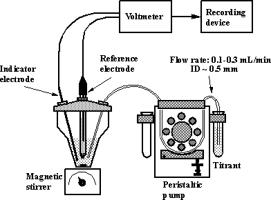
Fig.1-2 Experimental setup for a potentiometric titration using a peristaltic pump as titrator.

1.5. Location of end point

There are several methods of end-point determination. We shall mention only few of them.

For potentiometric indicating system with a reference electrode (Fig.1-3) the end point is determined from the first derivative of the titration curve. For the indicating system with two identical electrodes, the end point is determined directly from the titration curve.

It is advised to attempt to estimate the end point with a precision of 0.2% or better.

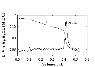
Fig.1-3 Titration and derivative curves for determination of Ca²⁺ with EDTA.

Sample: 1 ml drinking water; titrant: 5 mM EDTA; pH 10.5; total volume ~5 ml; indicating electrode: mercury-coated silver electrode, reference electrode: Ag/AgCl/1 M KCl.

(Data from Exp.1 in section "Potentiometric titrations").

Repetitive-monotonic mode of titration

In continuous follow-up of the progress of a titration, the main problem is the slow response of the electrodes, mainly in the vicinity of the end point. In commercial instrumentation the rate of titration is decreased when approaching the end point. A different (simpler) approach is proposed here.

The titration is carried out at constant rate (constant generating current). Due to the slow response of the electrode, the end point lags behind the equivalence point. Performing a series of titrations by adding the sample to the previously titrated solution solves the problem (Fig.1-4). The distance between the successive end points corresponds to the true value of the end-point time. (This is correct only for cases in which the response of the electrodes does not change from titration to titration).

Fig.1-4 Repetitive-monotonic coulometric titration of chlorides.

Initial composition: 0.500 ml 5.10 mM NaCl, 0.25 ml 1.2 M HClO₄, 4 ml methanol.

Generating electrodes: a mercury-coated silver wire and a small-area tungsten electrode (0.1 cm²); i_g = 2 mA.

Potentiometric indicating system: twin mercury-coated silver wires, i_ind = 2 mA.

End-point times are printed; first end point is delayed. Arrows correspond to new additions of analyte.

Treatment of potentiometric titration curves for the case of incomplete reactions at the equivalence point. Gran's approach

The end point in a potentiometric titration is taken as the inflection point of the titration curve. At low concentration of analyte or insufficiently large equilibrium constant, the degree of incompleteness of the reaction is highest around the equivalence point (why?).

Gran's approach is based on transformation of the potentiometric plot (in which the signal is a logarithmic function of the concentration) to a plot where the transformed function is linear in concentration. Extrapolation of the linear part enables a more accurate determination of the end point. Different types of transformation are available in the literature.

Example of Gran's treatment is presented in Fig.1-5. V_t/V_in is a correction for the dilution. (V_t is the volume of the titrated solution in the cell at a given time t, V_in is the initial volume in the cell prior to the start of the titration).

Fig.1-5 Determination of bicarbonates in drinking water.

Sample: 5 ml tap water from Tel-Aviv University. Titrant: 10.00 mM HCl.

We shall apply the Gran treatment to the potentiometric titration of a weak base (bicarbonate) with strong acids.

(1)

The titration is conducted by measuring the pH with a glass electrode.

The titration curve, expressed as pH or E vs volume of titrant, yields an S-shape plot. The end point is determined from data around an ill-defined inflection point (the later results from an incomplete reaction between the weak base and the strong acid; cf., Fig.1-5, left). If however, the titration curve is displayed as [H⁺] vs volume of titrant, it consists of a pair of straight lines, with the end point at the intersection of the two branches (Fig.1-5, right).

The form of the [H⁺]/volume plot is explained as follows. Previous to the end point, [H⁺] is virtually zero and the left branch of the titration curve is a straight line with zero slope. In the vicinity of the end point the plot is curved, due to the incompleteness of the reaction. Beyond the end point the carbonic acid is totally undissociated and the concentration of H⁺ is proportional to the number of moles of H⁺ added, yielding a rising straight line. The advantage of the right-side plot in Fig.1-5 is obvious.

The transformation from one type of titration display to another is achieved using eq.2:

(2)

where k’ is a constant, s is equal to (2.3RT/F) and f_H⁺ is the activity coefficient.

From eq. (2): , where

For applying the treatment, k and s should be accurately known. These quantities can be determined from a blank titration, performed under conditions similar to those of the sample titration (temperature, ionic strength, flow rate of titrant, etc.) and as near as possible to the time of the main titration.

1.6. Operation with low flow-rate pumps

Calibration: determination of the flow rate. The exact amount of titrant used in a titration is calculated upon the value of flow rate of the pump and the time of titration. The calibration consists of determination of the flow rate of the pump and represents the amount of liquid transferred through the flexible pump tube during a measured period of time. It is recommended to perform the calibration as near as possible to the time of the analysis. To achieve a statistically acceptable result, the measurement must be repeated several times. The values of the mean and the standard deviation (STD) of such group of measurements are the important factors, which mainly determine the precision of the method. In the case of a peristaltic pump the flow rate should be measured frequently due to changes in physical properties of the flexible tubing.

The arrangement used for calibration is shown in the figure below. Two 10-ml plastic test tubes are located at both sides of the pump: one of them is filled with deionized water, the other (the recipient vessel) is empty. A flexible pump tube connects between the two test tubes. Note, that one end of the flexible tube is dipped into the water, while the other end is placed into an additional small Teflon tube and touches its inside wall. The purpose of the small Teflon tube is to prevent loss of liquid while removing the pump tube at the end of the measurement.

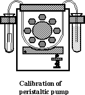
To perform the calibration, place the recipient vessel (the empty 10-ml test tube with the small Teflon tube inside) in a beaker and weigh both of them. Gently touch the end of the pump tube with soft tissue to remove excess of liquid. Insert carefully the end of the pump tube into the Teflon tube. Turn the pump on and transfer deionized water for a predetermined time (~1 min). Stop the pump and remove the pump tube from the recipient test tube. Weigh again. Calculate the flow rate in g/min and ml/min. Repeat the calibration three more times.

Operating parameters for peristaltic pump. The required flow rate of titrant is achieved by choosing the proper tubing size and rotation rate of the peristaltic pump. For optimal operation the pressure applied on the flexible tube is chosen in the plateau region of the experimental plot in Fig.1-6. The shape of the plot depends on size and type of tubing material.

Fig.1-6 Effect of pressure applied by the micrometer screw on the flexible tube of a peristaltic pump.

Adding the titrant. Remove any drops on the outside of the pump tube with absorbent tissue and insert the tube into the titrant. To fill the pump tube with the titrant turn the pump on and let the titrant flow through the tube for about 30 s.

At the end of the working session the pump tube should be rinsed with distilled water. Rinse the free end of the tube with water. Dip it into distilled water and operate the pump for several minutes. For the peristaltic pumps after rinsing the tube release the tension on the tube. This prolongs its life.

1.7. Cell

The geometry of the titrating cell is of lesser importance in point-by-point titrations. However, for automatic mode of titrations several requirements should be fulfilled. The stirring should be efficient, but smooth. Vortexes and air bubbles should be avoided in order to keep the relevant parts of the sensor in constant touch with the solutions. 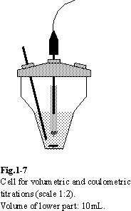The volume of the solution in the cell and the intensity of the stirring should be such as to ensure efficient transport throughout the solution. The cell shown in Fig.1-7 is found to be convenient for automatic titrations (in this specific cell the volume of the solution should not extend beyond the lower part of the cell).

Components inserted into the cell should not touch the cell walls or each other. Such situation would cause formation of pockets of stagnant solution, perturbing the distribution of reactants. In volumetric titrations the tip of the burette (Teflon tube with inner diameter not larger than 0.8 mm or antidiffusional microvalves) should be dipped into the analyte solution, but not in the immediate vicinity of the indicator electrodes. It is important to position it in the bottom part of the cell to ensure fast mixing of the titrant. The tip, if not antidiffusional, should be inserted just before the start of the titration.

Reference

1. D. Tzur and E. Kirowa-Eisner, Anal. Chim. Acta, 355, 85(1997).

Recommended Literature

1. D. A. Skoog, Principles of Instrumental Analysis.

2. D. A. Skoog and D. M. West, Principles of Instrumental Analysis.

3. D. A. Skoog and J. J. Leary, Instrumental Analysis.

4. D. C. Harris, Quantitative Chemical Analysis.

5. G. D. Christian, Analytical Chemistry.

Go to Main Page