Jacobian

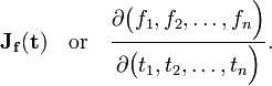
In mathematics, the Jacobi matrix is the matrix of first-order partial derivatives of the (vector-valued) function:
(often f maps only from and to appropriate subsets of these spaces). The Jacobi matrix is m × n, i.e., consists of m rows and n columns. Row k contains the first-order partial derivatives of fk with respect to x1, ...,xn, respectively. The Jacobi matrix is also known as the functional matrix of Jacobi. The determinant of the Jacobi matrix for n = m is known as the Jacobian. The Jacobi matrix and its determinant have several uses in mathematics:
- For m = 1 (f is a scalar valued function of n variables), the Jacobi matrix appears in the second (linear) term of the Taylor series of f. Here the Jacobi matrix is 1 × n (the gradient of f, a row vector).
- The Jacobian appears as the weight (measure) in multi-dimensional integrals over generalized coordinates, i.e, over non-Cartesian coordinates.
- The inverse function theorem states that if m = n and f is continuously differentiable, then f is invertible in the neighborhood of a point x0 if and only if the Jacobian at x0 is non-zero.
The Jacobi matrix and its determinant are named after the German mathematician Carl Gustav Jacob Jacobi (1804 - 1851).
Contents |
[edit] Definition
Let f be a map of an open subset T of  into
into  with continuous first partial derivatives,
That is if

then
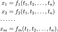
with

The m × n functional matrix of Jacobi consists of partial derivatives
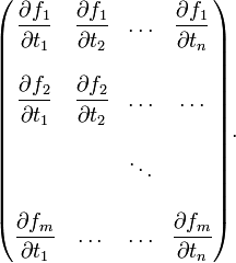
The determinant (which is only defined for square matrices) of this matrix is usually written as (take m = n),
[edit] Example
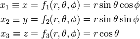
Let T be the subset {r, θ, φ | r > 0, 0 < θ<π, 0 <φ <2π} in ℝ3 and let f be defined by
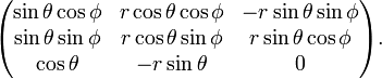
The Jacobi matrix is
Its determinant can be obtained most conveniently by a Laplace expansion along the third row
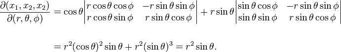
The quantities {r, θ, φ} are known as spherical polar coordinates and its Jacobian is r2sinθ.
[edit] Coordinate transformation
Let  . The map
 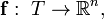 is a coordinate transformation if (i) f has continuous first derivatives on T (ii) f is one-to-one on T and (iii) the Jacobian of f is not equal to zero on T.
[edit] Multiple integration
It can be proved [1] that
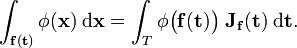
As an example we consider the spherical polar coordinates mentioned above. Here x = f(t) ≡ f(r, θ, φ) covers all of  , while T is the region {r > 0, 0 < θ<π, 0 <φ <2π}. Hence the theorem states that
[edit] Geometric interpretation of the Jacobian
The Jacobian has a geometric interpretation which is illustrated for the example n = 3.
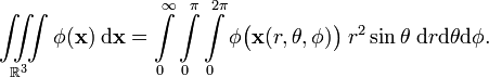
The following is a vector of infinitesimal length in the direction of increase in t1,

Similarly, we define
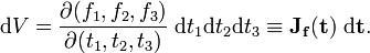
The scalar triple product of these three vectors gives the volume of an infinitesimally small parallelepiped,
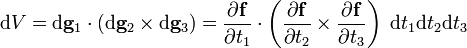
The components of the first vector are given by
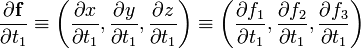
and similar expressions hold for the components of the other two derivatives. It has been shown in the article on the scalar triple product that
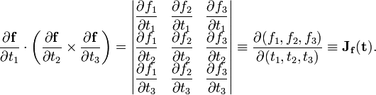
Note that a determinant is invariant under transposition (interchange of rows and columns), so that the transposed determinant being given is of no concern. Finally.
[edit] Reference
- ↑ T. M. Apostol, Mathematical Analysis, Addison-Wesley, 2nd ed. (1974), sec. 15.10