ARE MAGNETIC FIELD LINES CLOSED?
(7/98) Y. Kantor: I have attempted to summarize the subject, and our readers
are welcome to judge!
(June 8 and 10, 1998) Michael Trott wrote (slightly edited):
It does not follow from the equation div B=0, that field lines are closed.
Actually if you write down the explicit equation for the field
lines together with the maxwell equation, then they can be cast into
the form of Hamilton's equations and then we are on save ground to
decide if the trajectories are closed. Only for pure 2D current
arrangements the system is integrable. Details can be found in:
E. Petrisor. Physica D 112, 319 (1998)
J. R. Cary, R. G. Littlewood. Ann. Phys. 151, 1 (1983)
E. Pina. J. Phys. A 21, 1293 (1988)
J. Slepian. Am. J. Phys. 19, 87 (1951)
G. F. T. del Castillo. J. math. Phys. 36, 3413 (1995)
V. Arnold. C.R. Acad. Sci. Paris 261, 17 (1965)
A. F. Ranada. Phys. Lett. A 232, 25 (1997)
Actually it takes a few minutes of playing around on a computer to
discover this. Just take any closed 3d loop (not planar), calculate
B via Biot-Savart and integrate the field line equations. They do
not close.
Doing a numerical integration for knotted coils then gives you
quite some surprises in the shape of the field lines too. They are
never restricted to the inside of the coil, they always 'escape'
somewhere.
(June 20, 1998) The response of Christian von Ferber was as follows:
We here give account of some numerical investigation concerning the existence
and creation of knotted magnetic field lines by a current and finally give
an argument of how to create a magnetic field line along a predescribed
curve.
A numerical study
A trefoil knot may be parameterized in the following way:
x(t)= -10*cos(t)-2*cos(5*t)+15*sin(2*t)
y(t)= -15*cos(2*t)+10*sin(t)-2*sin(5*t)
z(t)= 10*cos(3*t)
t=0..2*pi
Along this line we center current loops of radius a=1 with
face perpendicular to the line.
We calculate the magnetic field as a superposition of the known solution
for a single current loop [e.g. Landau,Lifshitz Vol.8].
We increase the number N of current loops. The field strength
H at the center of the loops normalized by N approaches
a limit H/N -> h.
To achieve sufficient accuracy (10-6) we use 500 loops
placed equidistantly along the parameter values t.
We integrate the resulting field in real space steps of eps=10-3.
After 230,000 steps the field line we followed came
back to its origin within 0.04 . This is to be compared with the
radius a=1.0 of the 'solenoid'. We have at this point not checked
whether the accuracy may be increased further. Obviously decreasing eps
may at the same time increase rounding errors.
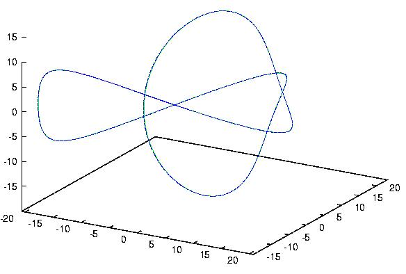
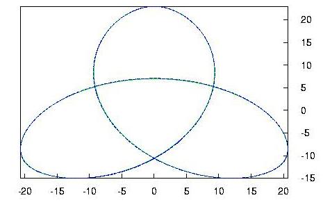
Find here a plot of the trefoil (center of the solenoid in green) and
the integrated solution (in blue) from two different viewpoints:
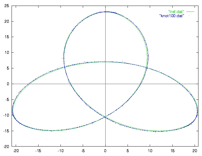
To check if the field lines might escape the solenoid we have also performed
a less time consuming integration with the step length eps=0.1. We
followed some 100 revolutions along the solenoid without
finding signs of serious divergence of the curve. We plot here every 100th
point of this integration in blue along with the trefoil line in green:
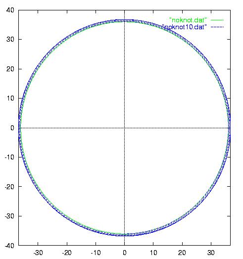
The Zero - Knot: A toroidal solenoid
To get some idea about the influence of the numerical errors we have performed
the same procedure as above also on the toroidal solenoid, for which the
exact solution is known. To receive similar dimensions we have used
a torus with centerline along a circle of radius R=36. This
implies an arc length of this line of about L=226 comparable to
the arc length of the trefoil knot above. Along this line we have again
placed N=500 current loops each of radius a=1. The result
of the integration with step length eps=10-1 was similar
to the integration along the trefoil line. (see below for 10 revolutions).
Integrating with high precision (eps=10-3) we find that the field
line along the centerline returns to its origin within a distance of 0.004
e.g. some 1/10th of the error found in the knotted configuration.
This might be an indication, that indeed the field line in the knotted
configuration does not close, but is still far from a proof, which may
not be provided numerically.
How to generate a closed knotted magnetic field line
We have seen above that the N current loops aligned along the
trefoil curve do not suffice to guarantee that there is a field line along
the predescribed curve. But also we know from the numerical experiments
that we need only some small correction. We may thus place at each of the
N points two additional current loops centered at the same point
but each with some individual small angle to the curve. Choosing the current
strengths in these loops while keeping the angles fixed gives us 2N
degrees of freedom. This is enough to align the magnetic field at
each of the N points with the curve (also 2N degrees
of freedom). As the magnetic field is a linear superposition of the now
3N current loops it is even a linear problem which will be nondegenerate
if the angles of the additional loops are properly chosen (the 3 loops
at each point should have non-coplanar directions). Including even the
choice of the angles it is clear that more that sufficient degrees of freedom
exist to produce a magnetic field line along any predescribed smooth curve.
(June 22, 1998) The reply of Michael Trott was as follows:
I disagree with the conclusion.
-As long as you take a finite number of turns you must connect the
loops and this gives a very thiny contribution to the magnetic field
which is not in the direction parallel to the knots local tangent.
-Also if you write out the equations for the corresponding
Hamiltonian system for the single loops along the knot, I highly
doubt that it will be integrable for any field line other then the
one in the center (if at all).
(June 22, 1998) Christian von Ferber's reply:
Of course, we are here coming close to splitting hairs, but let me add
that taking full control over the complete configuration of the wire,
rather than constraining it to just connecting the loops, gives me even
more degrees of freedom which can be used to refine the contour of the
magnetic field. The argument of the 3N loops was more thought of being
directly convincing, as it leads to a linear equation.
More generally one may use the dense winding limit (which is standard
when considering solenoids). Then one may think of the solenoid as a
tube around the given (knotted) line. Along this tube we now have full
control of the shape of its surface plus the density of winding along
the tube. obviously this gives us per point on the line an infinity of
degrees of freedom, while we only have to fix two degrees of freedom to
align the magnetic field there. It seems that this should even suffice
to align a bunch of lines of non-zero measure around this line.
But even if we had only this one closed magnetic field line, this would
correspond to a `bound state' solution in an otherwise non-integrable
Hamiltonian system. In fact these solutions are of some importance when
one considers the quantized version of such systems -- I know people who
like to count them, but this may be a matter of attitude.
(7/98) Y. Kantor: I think that the argument reached a point where only
a clear analytical argument can change the opinions of people. We welcome
such arguments...