See Path Segmentor module:
SEE Path Segmentor is a software designed to segment Open Field data into sequences of stops (lingering episodes) and progression segments. The input files for this module are the output files of See Path Smoother (“.txt” files).
See Path Segmentor applies the EM (Expectation-Maximization) algorithm to fit a gaussian mixture model to the frequency distribution of maximal speeds of the animal’s motion segments (segments of motion between stops). This procedure provides an intrinsic criterion for sorting motion segments into two groups: lingering segments (in which low maximal speeds are attained) and progression segments (movesegments) in which high maximal speeds are attained.
Instructions for program use:
- Upload data files if necessary. Use the ‘Add..’ button In the SEE Workshop window and select the directory of the folder of the relevant input files (i.e. the files which are the output of the smoothing stage).
Note:
· See Path Segmentor (as all the other modules of SEE Workshop will process all files in the folder).
· This folder will also be the folder where the output files are created.
- Set the ‘SEE Path Segmentor’ as follows:
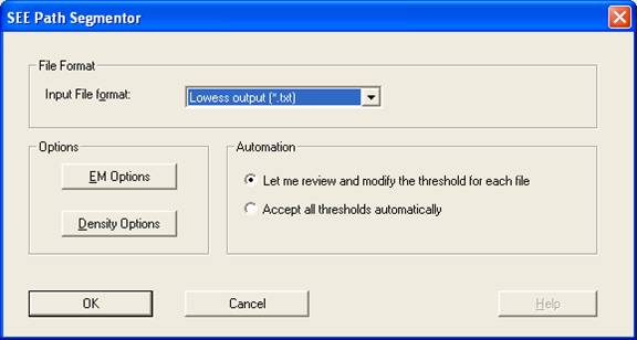
- Choose the desired input File format:
- Smoothed data (*.txt): Output of SEE Path Smoother.
- Mathematica List (*.lst): A list imported from Wolfram's Mathematica™ program.
- Set the EM Options parameters:

- Number of gaussians: The considerations for choosing the number of gaussians in the EM algorithm are rather involved and will be explained in a later help version of this program. We presently use as default 2 gaussians.
- Number of iterations: We find 2000 iterations to be sufficient.
- Set the Density Options parameters:

- Max Velocity Transformation: The transformation of segment maximal velocities may be needed in order to improve the fitting of the Mixed Gaussian Model to the distribution of the velocity data. We presently recommend the Log(2+x) transformation for mouse behaviour phenotyping.
- Density Plot Properties: Influences only the graphical visualization of the density (it does not affect the EM algorithm). The recommended value is 0.2 cm/sec.
- Cut Off Value: In order to separate between the modes of speeds, we would like to disregard motion segments whose maximum speed value lies within the system noise range due to inability to distinguish between real behavior and system noise. The proper cut-off-value depends on the set-up that you use. Tracking a still object in several locations in the arena can retain a good estimation of the system noise. [[Our noise threshold is 1 cm/sec in the center and ~2.5 cm/sec in the perimeter]]. If the parameters of the running medians (see path smoother) are well adjusted, there may be no need in using the cut off value, and the value to be inserted is 1e-006 (a value close to zero).
- Press the OK buttons and the Process button on the SEE Workshop window.
- Verify that only the desired checkboxes are marked.
- For each input file a Density Visualization dialog box will be opened (see below). This dialog box is used to interactively generate the cut off speed (threshold) that distinguishes between lingering episodes (staying in place) and progression segments (movesegments). Once the threshold is approved by the user, the setup information file ".inf" is updated.
- Density Visulaization Dialog Window:
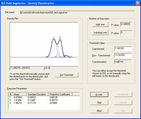
The dialog box presents a visualization of the ‘max
velocities’ density plot along with a superimposed graph of the
Density Plot: The plot presents the density of the
max velocity within motion segments (in black), the
o Dan Drai, Yoav Benjamini, Ilan Golani (2000) Statistical discrimination of natural modes of motion in rat exploratory behavior. Journal of Neuroscience Methods 96(2): 119-131.
Note:
·
The density function is performed
on the transformed data (according to the Max Velocity Transformation
that was chosen). The density graph and the parameters of the fitted Gaussians
can be affected substantially by the selected transformation.
Threshold Value: The threshold value that was chosen by the program appears in the "Transformed" and "Non-Transformed" edit boxes. The non-transformed value allows the user to use his intuition and judgment for either accepting the threshold or setting it manually. The default is accepting the threshold suggested by the program by clicking on the Accept button. To set the threshold manually, you can:
1. Type the desired value into the "Non-Transformed" edit box.
2. Use the mouse cursor to point the desired X-coordinate on the density plot, and click the mouse. The selected X,Y coordinates appear under the plot, on the right. Once you are satisfied with the selected X coordinate, press the Set Threshold button.
Number of Gaussians: We recommend the use of a 2 Gaussians model for mouse phenotyping. The program allows, however, changing the number of Gaussians in the fitted Gaussian mixture model by clicking the buttons Add +1 and Reduce –1. The two P value windows next to these buttons show the p value for the improvement in fit between the currently used Gaussian mixture model and a model that contains one more or one less Gaussians respectively. When the improvement in fit for adding a Gaussian becomes insignificant (p value of more than 0.05), then there is no need to increase further the number of Gaussians.
Gaussian Parameters: This section shows the parameters (mean, standard deviation and proportion coefficient) for each of the Gaussians in the Gaussian mixture model that is fitted to the data. For further reading on the Gaussian parameters, the interested reader is referred to the paper given above:
Once you are satisfied with the number of Gaussians and the selected threshold, press the Accept button. The threshold will be inserted into an “.inf” file.