Basic Biostatistics

Statistical Studies in Populations

In order for a study to be performed, the population must be defined. When one studies the extent of diabetes mellitus amongst the Hispanic population of Los Angeles, does that mean both males and females, adults only, persons who have emigrated from Latin America, persons who live just in the city of Los Angeles, etc? One must be very careful about defining the population to be studied.

Since it is not practical to perform tests or measures on all members of a population, then one must obtain a sample of that population. There are methods available to randomize the sampling of the population. The closer the measurements are to the "real" or true value for a population, the more unbiased the study. Precision in a study simply refers to how repeatable it is. The larger the sample, the more precise the study.

Example of a study:

You are conducting a health screening program in a community. You obtain a series of findings for a set of persons attending the program. This study includes adult men and women between the ages of 20 and 76 on a particular day in a particular community. This population is not narrowly defined. The results are as follows:

Distribution and Central Tendency:

A measure of the probability of a distribution of values is known as the central tendency and can be simply calculated as a mean, median, or mode:

Mean: This is the sum of a list of numbers, divided by the total number of numbers in the list. It is also called the arithmetic mean.

Median: This is the middle value in a list and is the smallest number such that at least half the numbers in the list are no greater than it. If the list has an odd number of entries, the median is the middle entry in the list after sorting the list into increasing order. If the list has an even number of entries, the median is equal to the sum of the two middle (after sorting) numbers divided by two.

Mode: For lists, the mode is the most common (frequent) value. A list can have more than one mode.

The range of values gives an indication of distribution of values and is just the highest value minus the lowest value.

In the above set of patients:

1. What is the mean for the glucose?

Measurement of Variability

Variability occurs in a set of values. Variability is the amount of distribution of values away from central tendency. Measures of the deviation of values from the central tendency can include the variance and the standard deviation.

Variance is the average of the squared deviations from the arithmetic mean. The standard deviation is a square root from variance value. The standard deviation is a measure of the variability of values around the mean and is meant to be used with values that are normally distributed (e.g., follow a normal curve). The standard normal curve is a bell-shaped curve. Non normal (skewed) data can sometimes be transformed to give a graph of normal shape by performing some mathematical transformation (such as using the variable's logarithm, square root, or reciprocal). Some data, however, cannot be transformed into a smooth pattern. The data for height and weight are "positively" skewed because such measures do not approach zero.

Skewed distributions have a median that lies to the left or right of the mean. A measurement of the amount of skew can be given by the formula:

skew = 3(mean - median)/SD

In the above distribution of glucose values, the mean of 105 is slightly greater than the median of 101, so the skew is +0.5, or very slightly skewed to the right.

For most bell-shaped curves, 68% of the values fall within 1 standard deviation of the mean, 95% within 2 SD's, and 97.7% within 3 SD's. For most laboratory tests, the "normal range" is defined as values falling within 2 SD's of the mean. This is sometimes called the "95% confidence limits". In general, a "significant" P value of <0.05 corresponds to a 95% confidence limit. It is not possible to know the exact population mean, because we cannot perform measurements on everyone, but we can take a sample (preferably large) of persons to try and estimate the population mean.

For bigger numbers for a set of values, the standard deviation is bigger, but does this imply that the values are more variable than for a set of values with a smaller mean? The coefficient of variation can be calculated to determine this variability when comparing two sets of data with different means. The CV is calculated as the SD divided by the mean and multiplied by 100.

5. What is the standard deviation for glucose values?

Another measure is the "standard error of the mean" or just standard error (SE) which is calculated as the standard deviation of each set of values divided by the square root of the number of the observations in the sample.

7. What is the standard error (SE) for glucose in the above patients?

Confidence Limits and the t Test

The 95% confidence limits are typically 2 SD's from the mean for a large sample size, typically over 60 values. For smaller sample sizes, such as the one above, there is more likely to be variation from the mean. For analyzing the variance and estimating the standard deviation for a small sample, the "student" or "t" test is done. In such a test, the number of "degrees of freedom" is calculated, which is the sample size minus one, or 14 for the above group. One then uses a table of pre-calculated values for different confidence limits for different degrees of freedom. In the table, for 14 degrees of freedom at 0.05 probability, the value is 2.145. Thus, the 95% confidence limits would be 2.145 SD's from the mean, or slightly more than the 2 SD's for a larger group.

The "t" test is a "two-tailed" test because the "tail" of the distribution on each side of the mean is analyzed. For many laboratory measurements or clinical trials, one would want a two tailed test because the value or the outcome could be either above or below the mean.

Note that the above set of patients has a mean, 105 mg/dL, and a SD, 22 mg/dL, which are much larger than for a typical "normal" population in which the mean is usually 90 mg/dL and the SD 10 mg/dL. Thus, the typical "normal range" for glucose is given as 70 to 110 mg/dL.

What is the likelihood that the populations are, indeed, different, and our population is abnormal compared to the "normal" population from which the normal range was calculated? The difference in means is 15 mg/dL, and the standard error of the mean for our population is 5.7 mg/dL. Dividing the former by the latter gives a "z" value of 2.63, which is more than 2 SD's, and therefore beyond the 95% confidence limits, so our sample study group is different from the normal population. This is a "one sample t test" because it measures the difference of sample mean from the population mean.

A t test comparing the difference in the means of two samples can also be calculated with a more complex formula. A "paired t test" can be performed using matched sets of data from a study group and a control group, for example.

A "Chi-square" test can be done to compare sets of observations, classically arranged in a "2 X 2" table, as in the comparison of compliance with two different treatment plans (two columns for compliance and non-compliance; two rows for treatment A and for treatment B). There can be more columns and rows, but the math gets more complex. A comparison is made of observed and expected values as follows:

Chi-square = sum of (observed - expected)2/expected

The degrees of freedom are calculated as: df = (rows -1)(columns - 1)

Thus, for a study comparing compliance with running and swimming as exercise regimens for weight maintenance, we might get the following data:

8. What is the Chi-square for this study and what is the significance?

Correlation and Regression

An association between data can be determined by a correlation coefficient. This can be done if the relationship is linear. It is often the case that a scatter plot of data comparing two measurements is done. For the patients above, one can plot the relationship of weight to glucose, as follows: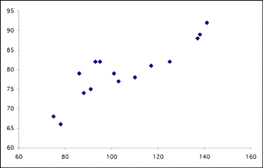

Looking at the plot suggests that the glucose is higher for persons who have a greater weight, but what is the correlation coefficient?

The correlation coefficient is measured on a scale that varies from + 1 through 0 to - 1. Complete correlation between two variables is expressed by either + 1 or -1. When one variable increases as the other increases the correlation is positive; when one decreases as the other increases it is negative. Complete absence of correlation is represented by 0.

The formula is a bit complex:

r = sum of paired (x)(y) - (n)(mean of x)(mean of y) / (n-1)(SD of x)(SD of y)

9. In the above case, what is the correlation coefficient?

t = r (square root of (n-2)/1 - r2)

10. In this case, what is t and what does it mean?

When the data on the x axis change as a function of data on the y axis, then there is a relationship known historically as "regression" and the "regression line" on a scatter plot is the line drawn through the dots that defines the amount of correlation. A line sloping at 45 degrees, with dots closer together, indicates better correlation, while a flat line indicates no correlation. Remember: correlation is NOT causation!

Covariance is a measure of how two data sets vary with respect to each other. Analysis of variance, or ANOVA, is the term given to the method of analysing data from two or more groups.

All statistical tests are either parametric (assuming the data were sampled from a particular type of distribution, such as a normal distribution) or non-parametric (no assumption of type of distribution is made). In general, parametric tests are better than non-parametric tests. Non-parametric tests generate a rank order of values and ignore the absolute differences between values. The statistical significance is more difficult to show with non-parametric tests.

Other Types of Distributions

In some clinical studies, results are recorded simply as positive or negative, with no gradation or quantification. Did the colon cancer therapy work or not? Data from such studies form what is called a "binomial" distribution. 95% confidence limits can be set for such a distribution, similar to a normal distribution.

The "Poisson" distribution is used to describe discrete quantitative data such as numbers of events when the size of the sample population is large but the probability of an event is small, though the number of events is moderate. An example is the number of deaths from a particular type of cancer in a community on a particular day.

"Null" hypothesis, type I error and type II error:

In comparing two sets of values from population groups, one can make the assumption that they will be the same. This is called the "null hypothesis". For most statistical studies the goal is to show that the null hypothesis is unlikely, so a difference which is greater than the limits set, and which we therefore regard as "significant", will make the null hypothesis unlikely.

To reject the null hypothesis when it is true is to make what is known as a type I error, or "alpha" error (a false positive). The level at which a result is declared significant is known as the type I error rate, often denoted by alpha.

If the null hypothesis is not rejected when there is a real difference between the groups, then this is known as a type II error, or "beta" error (a false negative).

More about studies:

The best type of study is the one that is performed prospectively. A retrospective study starts with diseased subjects and then examines for possible causes. The best example of a prospective study with patients is the randomised controlled trial in which the subjects with a disease are randomised to one of two (or more) treatments, one of which may be a control treatment. Randomization insures that treatment groups will be balanced with both known and unknown prognostic factors. The treatments tested in the study should be concurrent, with the tested and control treatments given over the same time frame. The subjects need to be compliant with the treatment in order to have valid outcomes.

A parallel group design is one in which treatment and control are allocated to different subjects in the study. One set of subjects typically receives a "placebo" treatment that appears identical to the study treatment, but without a real effect (such as an inert compound instead of a real drug).

The best study is double blinded so that neither the investigator nor the subjects in the study are aware of which treatment is given to which subject. This is easiest to do for drugs.

A crossover study measures the effects of two or more sequential treatments given to the same set of subjects. In such as study each subject acts as his or her own control, reducing the requirement for more subjects to serve as a control group. However, there may be a carry over effect from the first treatment to affect outcomes for the second treatment.

A cohort study follows initially disease free subjects over a period of time. During that time, some subjects are exposed to risk factors, such as alcohol consumption, and the outcomes are measured. The cohort may be defined as persons born in a particular year (making them all the same age), persons who lived in a particular community, or persons who worked in a particular place The outcome may be a particular disease state (cirrhosis) or death. The prevalence of the disease studied is known or can be estimated from the data. Cohort studies need large numbers of subjects studied for long periods of time to be valid. Here is an example of such a study examining the risk for developing diabetes mellitus with a risk factor of cheeseburger consumption in a cohort of persons born in 1940:

The risk for developing the disease for those exposed is: a / a + b
The risk for develolping the disease for those not exposed is: c / c + d

The "relative risk" or RR is the ratio of these: RR = a(a + b) / c(c + d)

11. What is the RR is this study for developing diabetes mellitus from eating cheeseburgers?

In a "case control" study, one defines a population with a particular disease and then finds a suitable control group without the disease. One then compares the two using a particular risk factor for the disease. The cases and the controls may be matched for variables such as age, sex, and race, but they may be unmatched. Here is an example of an unmatched case control study comparing the risk for esophageal adenocarcinoma in persons with GERD:

Unlike the cohort study, a relative risk is not used in a case control study, where the prevalence of the disease is not known, and the apparent prevalence is based upon the ratio of sample cases to controls. Instead, an "odds ratio" is computed as follows:

Odds Ratio = a X d / b X c

An odds ratio can give a reasonable estimate of the relative risk when the proportion of subjects with the disease is small.

12. What is the odds ratio for development of esophageal adenocarcinoma when GERD is present in this study?

A "cross-sectional" study includes subjects without reference to their history of exposure or to their disease. Instead, the cross-sectional study analyzes the cases prevalent at the time of the study. Such studies may be based upon methods of sampling of a population, such as questionnaires, but there are problems with true random sampling.

Prevalence and Incidence and Rate:

The prevalence of a disease is the proportion of a population that are cases at a point in time. For example, the prevalence of systemic lupus erythematosus may stated to be 7 per 1000. The group measured can be defined more narrowly, as: the prevalence of diabetes mellitus in women ages 50 to 60 is 7%.

The incidence of a disease is the rate at which new cases occur in a population during a specified period. For example, the incidence of influenza in the year 2001 is 20 per 1000 per year.

In general, prevalence is used to track diseases that are more chronic, while incidence is used for more acute conditions, such as infectious diseases, with a shorter course.

The incidence contributes to the prevalence. For example, if there were 12 women in 1000 diagnosed with breast cancer last year (the incidence) and there were 39 in the same population already diagnosed and known to be living with breast cancer, a tumor registry would then report the prevalence as 0.051.

A rate is the number of events per unit of population over a particular time span. An example of this is mortality. Mortality is the incidence of death from a disease. The crude mortality rate for a given year is stated as:

Crude Mortality Rate = (Number of deaths in a year / mid-year population) X 1000

An "age-specific" mortality rate can be given as:

ASMR = (Number of deaths in a specific age group / mid-year population of that group) X 1000

Probability:

This is a quantitative measure of uncertainty. For a coin flip, the probability of either heads or tails is 0.5. Probability is given a fraction between 0 and 1. A probability of 0 means that the event cannot occur; a probability of 1 means that an event will always happen. The probability of an event is the ratio of the number of outcomes that constitute the event to the total number of possible outcomes:

P(event) = (number of event outcomes ) / (number of total outcomes).

In case of tossing coin, the probability of getting heads is: P(head) = 1/2 = 0.5.

Randomization:

Patients in randomised trials are not a random sample from the population of people with the disease in question but are a highly selected set of patients who were available and were willing to participate. However, it is possible to randomize this set into treated and untreated groups so that any differences in outcomes between the two treatment groups are due solely to differences in the treatment to be studied.

Answers to Questions:

1. What is the mean for the glucose?

Answer: 105 mg/dL

2. What is the median weight?

Answer: 79 kg

3. What is the mode for height?

Answer: 170 cm

4. What is the range for systolic blood pressure?

Answer: 70 mm Hg

5. What is the standard deviation for glucose values?

Answer: 22 mg/dL

6. What is the CV for systolic B.P.? For diastolic?

Answer: The SD for systolic is 18 and for diastolic is 11, which appear considerably different, but the CV for systolic is 13.8 and for diastolic is 12.6, much closer, indicating that the two sets are not that much different in terms of variability.

7. What is the standard error (SE) for glucose in the above patients?

Answer: 5.7 mg/dL

8. What is the Chi-square for this study and what is the significance?

Answer: Computing the Chi-square gives a value of 1.7 + 0.9 + 1.6 + 0.8 = 4

This is more than the value of 3.841 given in a table of chi square values for 1 degree of freedom for a probability of < 0.05, so this difference between the groups is significant.

9. In the above case, what is the correlation coefficient?

Answer: r = 0.88

10. In this case, what is t and what does it mean?

Answer: t = 6.6

For 13 degrees of freedom, 6.6 is much larger than the value of 2.16 for a 0.05 probability, and larger than the value of 4.22 for a 0.001 probability. Thus, this correlation is significant.

11. What is the RR is this study for developing diabetes mellitus from eating cheeseburgers?

Answer: RR = 2

Of course, in reality there are multiple factors at work, and the risk for any one event is determined by many risks.

12. What is the odds ratio for development of esophageal adenocarcinoma when GERD is present in this study?

Answer: Odds Ratio = 7.6