SciPy is a collection of mathematical algorithms and convenience functions built on the Numeric extension for Python. It adds significant power to the interactive Python session by exposing the user to high-level commands and classes for the manipulation and visualization of data. With SciPy, an interactive Python session becomes a data-processing and system-prototyping environment rivaling sytems such as Matlab, IDL, Octave, R-Lab, and SciLab.
The additional power of using SciPy within Python, however, is that a powerful programming language is also available for use in developing sophisticated programs and specialized applications. Scientific applications written in SciPy benefit from the development of additional modules in numerous niche’s of the software landscape by developers across the world. Everything from parallel programming to web and data-base subroutines and classes have been made available to the Python programmer. All of this power is available in addition to the mathematical libraries in SciPy.
This document provides a tutorial for the first-time user of SciPy to help get started with some of the features available in this powerful package. It is assumed that the user has already installed the package. Some general Python facility is also assumed such as could be acquired by working through the Tutorial in the Python distribution. Throughout this tutorial it is assumed that the user has imported all of the names defined in the SciPy namespace using the command
>>> from scipy import *
|
Python provides the facility of documentation strings. The functions and classes available in SciPy use this method for on-line documentation. There are two methods for reading these messages and getting help. Python provides the command help in the pydoc module. Entering this command with no arguments (i.e. > > > help ) launches an interactive help session that allows searching through the keywords and modules available to all of Python. Running the command help with an object as the argument displays the calling signature, and the documentation string of the object.
The pydoc method of help is sophisticated but uses a pager to display the text. Sometimes this can interfere with the terminal you are running the interactive session within. A scipy-specific help system is also available under the command scipy.info. The signature and documentation string for the object passed to the help command are printed to standard output (or to a writeable object passed as the third argument). The second keyword argument of “scipy.info” defines the maximum width of the line for printing. If a module is passed as the argument to help than a list of the functions and classes defined in that module is printed. For example:
Another useful command is source. When given a function written in Python as an argument, it prints out a listing of the source code for that function. This can be helpful in learning about an algorithm or understanding exactly what a function is doing with its arguments. Also don’t forget about the Python command dir which can be used to look at the namespace of a module or package.
SciPy is organized into subpackages covering different scientific computing domains. Some common functions which several subpackages rely on live under the scipy_base package which is installed at the same directory level as the scipy package itself and could be installed separately. This allows for the possibility of separately distributing the subpackages of scipy as long as scipy_base package is provided as well.
Two other packages are installed at the higher-level: scipy_distutils and weave. These two packages while distributed with main scipy package could see use independently of scipy and so are treated as separate packages and described elsewhere.
The remaining subpackages are summarized in the following table (a * denotes an optional sub-package that requires additional libraries to function or is not available on all platforms).
| Subpackage | Description |
| cluster | Clustering algorithms |
| cow | Cluster of Workstations code for parallel programming |
| fftpack | FFT based on fftpack – default |
| fftw* | FFT based on fftw — requires FFTW libraries (is this still needed?) |
| ga | Genetic algorithms |
| gplt* | Plotting — requires gnuplot |
| integrate | Integration |
| interpolate | Interpolation |
| io | Input and Output |
| linalg | Linear algebra |
| optimize | Optimization and root-finding routines |
| plt* | Plotting — requires wxPython |
| signal | Signal processing |
| special | Special functions |
| stats | Statistical distributions and functions |
| xplt | Plotting with gist |
Because of their ubiquitousness, some of the functions in these subpackages are also made available in the scipy namespace to ease their use in interactive sessions and programs. In addition, many convenience functions are located in the scipy_base package and the in the top-level of the scipy package. Before looking at the sub-packages individually, we will first look at some of these common functions.
To begin with, all of the Numeric functions have been subsumed into the scipy namespace so that all of those functions are available without additionally importing Numeric. In addition, the universal functions (addition, subtraction, division) have been altered to not raise exceptions if floating-point errors are encountered1, instead NaN’s and Inf’s are returned in the arrays. To assist in detection of these events new universal functions (isnan, isfinite, isinf) have been added. In addition, the comparision operators have been changed to allow comparisons and logical operations of complex numbers (only the real part is compared). Also, with the new universal functions in SciPy, the logical operations (except logical_XXX functions) all return arrays of unsigned bytes (8-bits per element instead of the old 32-bits, or even 64-bits) per element2.
Finally, some of the basic functions like log, sqrt, and inverse trig functions have been modified to return complex numbers instead of NaN’s where appropriate (i.e. scipy.sqrt(-1) returns 1j).
With the command scipy.alter_numeric() you can now use index and mask arrays inside brackets and the coercion rules of Numeric are changed so that Python scalars will not upcast the results of operations. An example is shown below
The purpose of scipy_base is to collect general-purpose routines that the other sub-packages can use. These routines are divided into several files for organizational purposes, but they are all available under the scipy_base namespace (and the scipy namespace). There are routines for type handling and type checking, shape and matrix manipulation, polynomial processing, and other useful functions. Rather than giving a detailed description of each of these functions (which is available using the help, info and source commands), this tutorial will discuss some of the more useful commands which require a little introduction to use to their full potential.
Note the difference between iscomplex (isreal) and iscomplexobj (isrealobj). The former command is array based and returns byte arrays of ones and zeros providing the result of the element-wise test. The latter command is object based and returns a scalar describing the result of the test on the entire object.
Often it is required to get just the real and/or imaginary part of a complex number. While complex numbers and arrays have attributes that return those values, if one is not sure whether or not the object will be complex-valued, it is better to use the functional forms real and imag. These functions succeed for anything that can be turned into a Numeric array. Consider also the function real_if_close which transforms a complex-valued number with tiny imaginary part into a real number.
Occasionally the need to check whether or not a number is a scalar (Python (long)int, Python float, Python complex, or rank-0 array) occurs in coding. This functionality is provided in the convenient function isscalar which returns a 1 or a 0.
Finally, ensuring that objects are a certain Numeric type occurs often enough that it has been given a convenient interface in SciPy through the use of the cast dictionary. The dictionary is keyed by the type it is desired to cast to and the dictionary stores functions to perform the casting. Thus, >>> a = cast[’f’](d) returns an array of float32 from d. This function is also useful as an easy way to get a scalar of a certain type: >>> fpi = cast[’f’](pi).
Thre are some class instances that make special use of the slicing functionality to provide efficient means for array construction. This part will discuss the operation of mgrid, ogrid, r_, and c_ for quickly constructing arrays.
One familiar with Matlab may complain that it is difficult to construct arrays from the interactive session with Python. Suppose, for example that one wants to construct an array that begins with 3 followed by 5 zeros and then contains 10 numbers spanning the range -1 to 1 (inclusive on both ends). Before SciPy, you would need to enter something like the following >>> concatenate(([3],[0]*5,arange(-1,1.002,2/9.0)). With the r_ command one can enter this as >>> r_[3,[0]*5,-1:1:10j] which can ease typing in an interactive session. Notice how objects are concatenated, and the slicing syntax is (ab)used to construct ranges. The other term that deserves a little explanation is the use of the complex number 10j as the step size in the slicing syntax. This non-standard use allows the number to be interpreted as the number of points to produce in the range rather than as a step size (note we would have used the long integer notation, 10L, but this notation may go away in Python as the integers become unified). This non-standard usage may be unsightly to some, but it gives the user the ability to quickly construct complicated vectors in a very readable fashion. When the number of points is specified in this way, the end-point is inclusive.
The “r” stands for row concatenation because if the objects between commas are 2 dimensional arrays, they are stacked by rows (and thus must have commensurate columns). There is an equivalent command c_ that stacks 2d arrays by columns but works identically to r_ for 1d arrays.
Another very useful class instance which makes use of extended slicing notation is the function mgrid. In the simplest case, this function can be used to construct 1d ranges as a convenient substitute for arange. It also allows the use of complex-numbers in the step-size to indicate the number of points to place between the (inclusive) end-points. The real purpose of this function however is to produce N, N-d arrays which provide coordinate arrays for an N-dimensional volume. The easiest way to understand this is with an example of its usage:
Having meshed arrays like this is sometimes very useful. However, it is not always needed just to evaluate some N-dimensional function over a grid due to the array-broadcasting rules of Numeric and SciPy. If this is the only purpose for generating a meshgrid, you should instead use the function ogrid which generates an “open” grid using NewAxis judiciously to create N, N-d arrays where only one-dimension in each array has length greater than 1. This will save memory and create the same result if the only purpose for the meshgrid is to generate sample points for evaluation of an N-d function.
In this category of functions are routines for squeezing out length-one dimensions from N-dimensional arrays, ensuring that an array is at least 1-, 2-, or 3-dimensional, and stacking (concatenating) arrays by rows, columns, and “pages” (in the third dimension). Routines for splitting arrays (roughly the opposite of stacking arrays) are also available.
These are functions specifically suited for 2-dimensional arrays that were part of MLab in the Numeric distribution, but have been placed in scipy_base for completeness so that users are not importing Numeric.
There are two (interchangeable) ways to deal with 1-d polynomials in SciPy. The first is to use the poly1d class in scipy_base. This class accepts coefficients or polynomial roots to initialize a polynomial. The polynomial object can then be manipulated in algebraic expressions, integrated, differentiated, and evaluated. It even prints like a polynomial:
The other way to handle polynomials is as an array of coefficients with the first element of the array giving the coefficient of the highest power. There are explicit functions to add, subtract, multiply, divide, integrate, differentiate, and evaluate polynomials represented as sequences of coefficients.
One of the features that SciPy provides is a class vectorize to convert an ordinary Python function which accepts scalars and returns scalars into a “vectorized-function” with the same broadcasting rules as other Numeric functions (i.e. the Universal functions, or ufuncs). For example, suppose you have a Python function named addsubtract defined as:
>>> vec_addsubtract = vectorize(addsubtract)
|
returns a function which takes array arguments and returns an array result:
This particular function could have been written in vector form without the use of vectorize. But, what if the function you have written is the result of some optimization or integration routine. Such functions can likely only be vectorized using vectorize.
There are several other functions in the scipy_base package including most of the other functions that are also in MLab that comes with the Numeric package. The reason for duplicating these functions is to allow SciPy to potentially alter their original interface and make it easier for users to know how to get access to functions >>> from scipy import *.
New functions which should be mentioned are mod(x,y) which can replace x%y when it is desired that the result take the sign of y instead of x. Also included is fix which always rounds to the nearest integer towards zero. For doing phase processing, the functions angle, and unwrap are also useful. Also, the linspace and logspace functions return equally spaced samples in a linear or log scale. Finally, mention should be made of the new function select which extends the functionality of where to include multiple conditions and multiple choices. The calling convention is select(condlist,choicelist,default=0). Select is a vectorized form of the multiple if-statement. It allows rapid construction of a function which returns an array of results based on a list of conditions. Each element of the return array is taken from the array in a choicelist corresponding to the first condition in condlist that is true. For example
Some functions depend on sub-packages of SciPy but should be available from the top-level of SciPy due to their common use. These are functions that might have been placed in scipy_base except for their dependence on other sub-packages of SciPy. For example the factorial and comb functions compute n! and n!∕k!(n - k)! using either exact integer arithmetic (thanks to Python’s Long integer object), or by using floating-point precision and the gamma function. The functions rand and randn are used so often that they warranted a place at the top level. There are convenience functions for the interactive use: disp (similar to print), and who (returns a list of defined variables and memory consumption–upper bounded). Another function returns a common image used in image processing: lena.
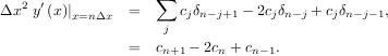
Finally, two functions are provided that are useful for approximating derivatives of functions using discrete-differences. The function central_diff_weights returns weighting coefficients for an equally-spaced N-point approximation to the derivative of order o. These weights must be multiplied by the function corresponding to these points and the results added to obtain the derivative approximation. This function is intended for use when only samples of the function are avaiable. When the function is an object that can be handed to a routine and evaluated, the function derivative can be used to automatically evaluate the object at the correct points to obtain an N-point approximation to the oth-derivative at a given point.
The main feature of the special package is the definition of numerous special functions of mathematical physics. Available functions include airy, elliptic, bessel, gamma, beta, hypergeometric, parabolic cylinder, mathieu, spheroidal wave, struve, and kelvin. There are also some low-level stats functions that are not intended for general use as an easier interface to these functions is provided by the stats module. Most of these functions can take array arguments and return array results following the same broadcasting rules as other math functions in Numerical Python. Many of these functions also accept complex-numbers as input. For a complete list of the available functions with a one-line description type >>>info(special). Each function also has it’s own documentation accessible using help. If you don’t see a function you need, consider writing it and contributing it to the library. You can write the function in either C, Fortran, or Python. Look in the source code of the library for examples of each of these kind of functions.
The integrate sub-package provides several integration techniques including an ordinary differential equation integrator. An overview of the module is provided by the help command:
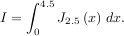
The function quad is provided to integrate a function of one variable between two points. The points can be ±∞ (±integrate.inf) to indicate infinite limits. For example, suppose you wish to integrate a bessel function jv(2.5,x) along the interval [0,4.5].
This could be computed using quad:
The first argument to quad is a “callable” Python object (i.e a function, method, or class instance). Notice the use of a lambda-function in this case as the argument. The next two arguments are the limits of integration. The return value is a tuple, with the first element holding the estimated value of the integral and the second element holding an upper bound on the error. Notice, that in this case, the true value of this integral is

where
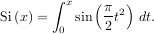
is the Fresnel sine integral. Note that the numerically-computed integral is within 1.04 × 10⁻¹¹ of the exact result — well below the reported error bound.
Infinite inputs are also allowed in quad by using ±integrate.inf (or inf) as one of the arguments. For example, suppose that a numerical value for the exponential integral:
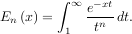
is desired (and the fact that this integral can be computed as special.expn(n,x) is forgotten). The functionality of the function special.expn can be replicated by defining a new function vec_expint based on the routine quad:
The function which is integrated can even use the quad argument (though the error bound may underestimate the error due to possible numerical error in the integrand from the use of quad). The integral in this case is

This last example shows that multiple integration can be handled using repeated calls to quad. The mechanics of this for double and triple integration have been wrapped up into the functions dblquad and tplquad. The function, dblquad performs double integration. Use the help function to be sure that the arguments are defined in the correct order. In addition, the limits on all inner integrals are actually functions which can be constant functions. An example of using double integration to compute several values of In is shown below:
A few functions are also provided in order to perform simple Gaussian quadrature over a fixed interval. The first is fixed_quad which performs fixed-order Gaussian quadrature. The second function is quadrature which performs Gaussian quadrature of multiple orders until the difference in the integral estimate is beneath some tolerance supplied by the user. These functions both use the module special.orthogonal which can calculate the roots and quadrature weights of a large variety of orthogonal polynomials (the polynomials themselves are available as special functions returning instances of the polynomial class — e.g. special.legendre).
There are three functions for computing integrals given only samples: trapz, simps, and romb. The first two functions use Newton-Coates formulas of order 1 and 2 respectively to perform integration. These two functions can handle, non-equally-spaced samples. The trapezoidal rule approximates the function as a straight line between adjacent points, while Simpson’s rule approximates the function between three adjacent points as a parabola.
If the samples are equally-spaced and the number of samples available is 2k + 1 for some integer k, then Romberg integration can be used to obtain high-precision estimates of the integral using the available samples. Romberg integration uses the trapezoid rule at step-sizes related by a power of two and then performs Richardson extrapolation on these estimates to approximate the integral with a higher-degree of accuracy. (A different interface to Romberg integration useful when the function can be provided is also available as integrate.romberg).
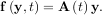
Integrating a set of ordinary differential equations (ODEs) given initial conditions is another useful example. The function odeint is available in SciPy for integrating a first-order vector differential equation:

given initial conditions y = y0, where y is a length N vector and f is a mapping from
  N to N. A
higher-order ordinary differential equation can always be reduced to a differential equation of this type by
introducing intermediate derivatives into the y vector.
N to N. A
higher-order ordinary differential equation can always be reduced to a differential equation of this type by
introducing intermediate derivatives into the y vector.
For example suppose it is desired to find the solution to the following second-order differential equation:

with initial conditions w =
=  and
and  z=0 = -
 . It is known that the solution to this differential
equation with these boundary conditions is the Airy function
. It is known that the solution to this differential
equation with these boundary conditions is the Airy function

which gives a means to check the integrator using special.airy.
First, convert this ODE into standard form by setting y = ![[dw-,w]
dz](tutorial13x.png) and t = z. Thus, the differential equation
becomes
and t = z. Thus, the differential equation
becomes
![dy [ty1 ] [0 t ][y0 ] [0 t ]
dt-= y0 = 1 0 y1 = 1 0 y.](tutorial14x.png)
In other words,
As an interesting reminder, if A commutes with ∫
0tA
commutes with ∫
0tA dτ under matrix multiplication, then this linear
differential equation has an exact solution using the matrix exponential:
dτ under matrix multiplication, then this linear
differential equation has an exact solution using the matrix exponential:

However, in this case, A and its integral do not commute.
There are many optional inputs and outputs available when using odeint which can help tune the solver. These additional inputs and outputs are not needed much of the time, however, and the three required input arguments and the output solution suffice. The required inputs are the function defining the derivative, fprime, the initial conditions vector, y0, and the time points to obtain a solution, t, (with the initial value point as the first element of this sequence). The output to odeint is a matrix where each row contains the solution vector at each requested time point (thus, the initial conditions are given in the first output row).
The following example illustrates the use of odeint including the usage of the Dfun option which allows the user
to specify a gradient (with respect to y) of the function, f .
.
There are several classical optimization algorithms provided by SciPy in the optimize package. An overview of the module is available using help (or pydoc.help):
The simplex algorithm is probably the simplest way to minimize a fairly well-behaved function. The simplex algorithm requires only function evaluations and is a good choice for simple minimization problems. However, because it does not use any gradient evaluations, it may take longer to find the minimum. To demonstrate the minimization function consider the problem of minimizing the Rosenbrock function of N variables:
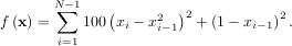
The minimum value of this function is 0 which is achieved when xi = 1. This minimum can be found using the fmin routine as shown in the example below:
Another optimization algorithm that needs only function calls to find the minimum is Powell’s method available as optimize.fmin_powell.
In order to converge more quickly to the solution, this routine uses the gradient of the objective function. If the gradient is not given by the user, then it is estimated using first-differences. The Broyden-Fletcher-Goldfarb-Shanno (BFGS) method typically requires fewer function calls than the simplex algorithm even when the gradient must be estimated.
To demonstrate this algorithm, the Rosenbrock function is again used. The gradient of the Rosenbrock function is the vector:


The calling signature for the BFGS minimization algorithm is similar to fmin with the addition of the fprime argument. An example usage of fmin_bfgs is shown in the following example which minimizes the Rosenbrock function.
The method which requires the fewest function calls and is therefore often the fastest method to minimize functions of many variables is fmin_ncg. This method is a modified Newton’s method and uses a conjugate gradient algorithm to (approximately) invert the local Hessian. Newton’s method is based on fitting the function locally to a quadratic form:

where H is a matrix of second-derivatives (the Hessian). If the Hessian is positive definite then the local
minimum of this function can be found by setting the gradient of the quadratic form to zero, resulting
in
is a matrix of second-derivatives (the Hessian). If the Hessian is positive definite then the local
minimum of this function can be found by setting the gradient of the quadratic form to zero, resulting
in

The inverse of the Hessian is evaluted using the conjugate-gradient method. An example of employing this method to minimizing the Rosenbrock function is given below. To take full advantage of the NewtonCG method, a function which computes the Hessian must be provided. The Hessian matrix itself does not need to be constructed, only a vector which is the product of the Hessian with an arbitrary vector needs to be available to the minimization routine. As a result, the user can provide either a function to compute the Hessian matrix, or a function to compute the product of the Hessian with an arbitrary vector.
The Hessian of the Rosenbrock function is


![[1,N - 2]](tutorial28x.png) with i,j
with i,j ![[0,N - 1]](tutorial29x.png) defining the N × N matrix. Other non-zero entries of the matrix are
defining the N × N matrix. Other non-zero entries of the matrix are

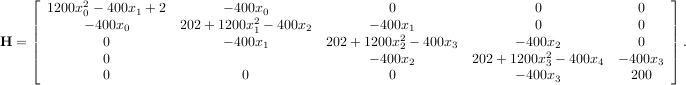
The code which computes this Hessian along with the code to minimize the function using fmin_ncg is shown in the following example:
For larger minimization problems, storing the entire Hessian matrix can consume considerable time and memory. The Newton-CG algorithm only needs the product of the Hessian times an arbitrary vector. As a result, the user can supply code to compute this product rather than the full Hessian by setting the fhess_p keyword to the desired function. The fhess_p function should take the minimization vector as the first argument and the arbitrary vector as the second argument. Any extra arguments passed to the function to be minimized will also be passed to this function. If possible, using Newton-CG with the hessian product option is probably the fastest way to minimize the function.
In this case, the product of the Rosenbrock Hessian with an arbitrary vector is not difficult to compute. If p is
the arbitrary vector, then H p has elements:

Code which makes use of the fhess_p keyword to minimize the Rosenbrock function using fmin_ncg follows:
All of the previously-explained minimization procedures can be used to solve a least-squares problem provided the
appropriate objective function is constructed. For example, suppose it is desired to fit a set of data
 to a known model, y = f
 where p is a vector of parameters for the model that need to be
found. A common method for determining which parameter vector gives the best fit to the data is to
minimize the sum of squares of the residuals. The residual is usually defined for each observed data-point
as
where p is a vector of parameters for the model that need to be
found. A common method for determining which parameter vector gives the best fit to the data is to
minimize the sum of squares of the residuals. The residual is usually defined for each observed data-point
as

An objective function to pass to any of the previous minization algorithms to obtain a least-squares fit is.

The leastsq algorithm performs this squaring and summing of the residuals automatically. It takes as an input
argument the vector function e and returns the value of p which minimizes J
 = eTe directly. The user is also
encouraged to provide the Jacobian matrix of the function (with derivatives down the columns or across the rows).
If the Jacobian is not provided, it is estimated.
= eTe directly. The user is also
encouraged to provide the Jacobian matrix of the function (with derivatives down the columns or across the rows).
If the Jacobian is not provided, it is estimated.
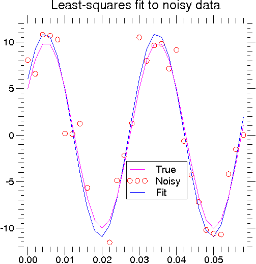
An example should clarify the usage. Suppose it is believed some measured data follow a sinusoidal pattern

where the parameters A, k, and θ are unknown. The residual vector is

By defining a function to compute the residuals and (selecting an appropriate starting position), the least-squares
fit routine can be used to find the best-fit parameters Â,  ,
,  . This is shown in the following example and a plot of
the results is shown in Figure 1.
. This is shown in the following example and a plot of
the results is shown in Figure 1.
Often only the minimum of a scalar function is needed (a scalar function is one that takes a scalar as input and returns a scalar output). In these circumstances, other optimization techniques have been developed that can work faster.
There are actually two methods that can be used to minimize a scalar function (brent and golden), but
golden is included only for academic purposes and should rarely be used. The brent method uses
Brent’s algorithm for locating a minimum. Optimally a bracket should be given which contains the
minimum desired. A bracket is a triple  such that f
 > f
> f < f
< f and a < b < c. If this is not
given, then alternatively two starting points can be chosen and a bracket will be found from these
points using a simple marching algorithm. If these two starting points are not provided 0 and 1 will be
used (this may not be the right choice for your function and result in an unexpected minimum being
returned).
and a < b < c. If this is not
given, then alternatively two starting points can be chosen and a bracket will be found from these
points using a simple marching algorithm. If these two starting points are not provided 0 and 1 will be
used (this may not be the right choice for your function and result in an unexpected minimum being
returned).
Thus far all of the minimization routines described have been unconstrained minimization routines. Very often, however, there are constraints that can be placed on the solution space before minimization occurs. The fminbound function is an example of a constrained minimization procedure that provides a rudimentary interval constraint for scalar functions. The interval constraint allows the minimization to occur only between two fixed endpoints.
For example, to find the minimum of J1 near x = 5, fminbound can be called using the interval
 ![[4,7]](tutorial50x.png) as a
constraint. The result is xmin = 5.3314:
as a
constraint. The result is xmin = 5.3314:
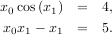
To find the roots of a polynomial, the command roots is useful. To find a root of a set of non-linear equations, the command optimize.fsolve is needed. For example, the following example finds the roots of the single-variable transcendental equation
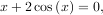
and the set of non-linear equations
If one has a single-variable equation, there are four different root finder algorithms that can be tried. Each of these root finding algorithms requires the endpoints of an interval where a root is suspected (because the function changes signs). In general brentq is the best choice, but the other methods may be useful in certain circumstances or for academic purposes.
A problem closely related to finding the zeros of a function is the problem of finding a fixed-point of a function. A
fixed point of a function is the point at which evaluation of the function returns the point: g = x. Clearly the
fixed point of g is the root of f
= x. Clearly the
fixed point of g is the root of f = g
= g - x. Equivalently, the root of f is the fixed_point of g
 = f
= f + x.
The routine fixed_point provides a simple iterative method using Aitkens sequence acceleration to estimate the
fixed point of g given a starting point.
+ x.
The routine fixed_point provides a simple iterative method using Aitkens sequence acceleration to estimate the
fixed point of g given a starting point.
There are two general interpolation facilities available in SciPy. The first facility is an interpolation class which performs linear 1-dimensional interpolation. The second facility is based on the FORTRAN library FITPACK and provides functions for 1- and 2-dimensional (smoothed) cubic-spline interpolation.
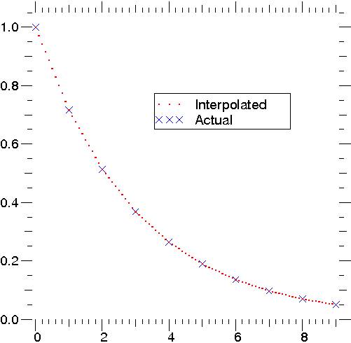
The linear_1d class in scipy.interpolate is a convenient method to create a function based on fixed data points which can be evaluated anywhere within the domain defined by the given data using linear interpolation. An instance of this class is created by passing the 1-d vectors comprising the data. The instance of this class defines a __call__ method and can therefore by treated like a function which interpolates between known data values to obtain unknown values (it even has a docstring for help). Behavior at the boundary can be specified at instantiation time. The following example demonstrates it’s use.
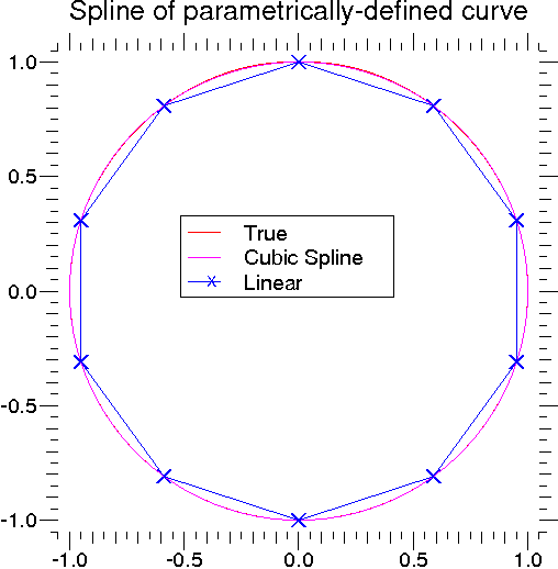
Spline interpolation requires two essential steps: (1) a spline representation of the curve is computed, and (2) the
spline is evaluated at the desired points. In order to find the spline representation, there are two different was to
represent a curve and obtain (smoothing) spline coefficients: directly and parametrically. The direct method finds
the spline representation of a curve in a two-dimensional plane using the function interpolate.splrep. The first two
arguments are the only ones required, and these provide the x and y components of the curve. The
normal output is a 3-tuple,  , containing the knot-points, t, the coefficients c and the order
k of the spline. The default spline order is cubic, but this can be changed with the input keyword,
k.
, containing the knot-points, t, the coefficients c and the order
k of the spline. The default spline order is cubic, but this can be changed with the input keyword,
k.
For curves in N-dimensional space the function interpolate.splprep allows defining the curve parametrically.
For this function only 1 input argument is required. This input is a list of N-arrays representing the curve in
N-dimensional space. The length of each array is the number of curve points, and each array provides one
component of the N-dimensional data point. The parameter variable is given with the keword argument, u,
which defaults to an equally-spaced monotonic sequence between 0 and 1. The default output consists
of two objects: a 3-tuple,  , containing the spline representation and the parameter variable
u.
, containing the spline representation and the parameter variable
u.
The keyword argument, s, is used to specify the amount of smoothing to perform during the spline fit. The
default value of s is s = m- where m is the number of data-points being fit. Therefore, if no smoothing is
desired a value of s = 0 should be passed to the routines.
where m is the number of data-points being fit. Therefore, if no smoothing is
desired a value of s = 0 should be passed to the routines.
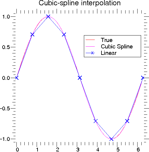
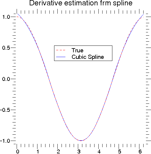
Once the spline representation of the data has been determined, functions are available for evaluating the spline (interpolate.splev) and its derivatives (interpolate.splev, interpolate.splade) at any point and the integral of the spline between any two points (interpolate.splint). In addition, for cubic splines (k = 3) with 8 or more knots, the roots of the spline can be estimated (interpolate.sproot). These functions are demonstrated in the example that follows (see also Figure 3).
For (smooth) spline-fitting to a two dimensional surface, the function interpolate.bisplrep is available. This
function takes as required inputs the 1-D arrays x, y, and z which represent points on the surface z = f .
The default output is a list
.
The default output is a list ![[tx,ty,c,kx,ky]](tutorial67x.png) whose entries represent respectively, the components of
the knot positions, the coefficients of the spline, and the order of the spline in each coordinate. It
is convenient to hold this list in a single object, tck, so that it can be passed easily to the function
interpolate.bisplev. The keyword, s, can be used to change the amount of smoothing performed on the data while
determining the appropriate spline. The default value is s = m -
whose entries represent respectively, the components of
the knot positions, the coefficients of the spline, and the order of the spline in each coordinate. It
is convenient to hold this list in a single object, tck, so that it can be passed easily to the function
interpolate.bisplev. The keyword, s, can be used to change the amount of smoothing performed on the data while
determining the appropriate spline. The default value is s = m - where m is the number of data points
in the x, y, and z vectors. As a result, if no smoothing is desired, then s = 0 should be passed to
interpolate.bisplrep.
where m is the number of data points
in the x, y, and z vectors. As a result, if no smoothing is desired, then s = 0 should be passed to
interpolate.bisplrep.
To evaluate the two-dimensional spline and it’s partial derivatives (up to the order of the spline), the function interpolate.bisplev is required. This function takes as the first two arguments two 1-D arrays whose cross-product specifies the domain over which to evaluate the spline. The third argument is the tck list returned from interpolate.bisplrep. If desired, the fourth and fifth arguments provide the orders of the partial derivative in the x and y direction respectively.
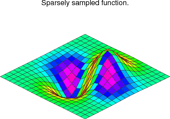
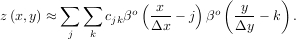
It is important to note that two dimensional interpolation should not be used to find the spline representation of images. The algorithm used is not amenable to large numbers of input points. The signal processing toolbox contains (soon) more appropriate algorithms for finding the spline representation of an image. The two dimensional interpolation commands are intended for use when interpolating a two dimensional function as shown in the example that follows (See also Figure 4). This example uses the mgrid command in SciPy which is useful for defining a “mesh-grid” in many dimensions. (See also the ogrid command if the full-mesh is not needed). The number of output arguments and the number of dimensions of each argument is determined by the number of indexing objects passed in mgrid[].
The signal processing toolbox currently contains some filtering functions, a limited set of filter design tools, and a few B-spline interpolation algorithms for one- and two-dimensional data. While the B-spline algorithms could technically be placed under the interpolation category, they are included here because they only work with equally-spaced data and make heavy use of filter-theory and transfer-function formalism to provide a fast B-spline transform. To understand this section you will need to understand that a signal in SciPy is an array of real or complex numbers.
A B-spline is an approximation of a continuous function over a finite-domain in terms of B-spline coefficients and knot points. If the knot-points are equally spaced with spacing Δx, then the B-spline approximation to a 1-dimensional function is the finite-basis expansion.

In two dimensions with knot-spacing Δx and Δy, the function representation is
In these expressions, βo is the space-limited B-spline basis function of order, o. The requirement of
equally-spaced knot-points and equally-spaced data points, allows the development of fast (inverse-filtering)
algorithms for determining the coefficients, cj, from sample-values, yn. Unlike the general spline interpolation
algorithms, these algorithms can quickly find the spline coefficients for large images.
is the space-limited B-spline basis function of order, o. The requirement of
equally-spaced knot-points and equally-spaced data points, allows the development of fast (inverse-filtering)
algorithms for determining the coefficients, cj, from sample-values, yn. Unlike the general spline interpolation
algorithms, these algorithms can quickly find the spline coefficients for large images.
The advantage of representing a set of samples via B-spline basis functions is that continuous-domain operators (derivatives, re-sampling, integral, etc.) which assume that the data samples are drawn from an underlying continuous function can be computed with relative ease from the spline coefficients. For example, the second-derivative of a spline is

Using the property of B-splines that

it can be seen that
![∑ [ ( ) ( ) ( )]
y′′(x) = -1-- cj βo-2 x--- j + 1 - 2βo- 2 -x-- j + βo-2 -x- - j - 1 .
Δx2 j Δx Δx Δx](tutorial76x.png)
If o = 3, then at the sample points,
The savvy reader will have already noticed that the data samples are related to the knot coefficients via a convolution operator, so that simple convolution with the sampled B-spline function recovers the original data from the spline coefficients. The output of convolutions can change depending on how boundaries are handled (this becomes increasingly more important as the number of dimensions in the data-set increases). The algorithms relating to B-splines in the signal-processing sub package assume mirror-symmetric boundary conditions. Thus, spline coefficients are computed based on that assumption, and data-samples can be recovered exactly from the spline coefficients by assuming them to be mirror-symmetric also.
Currently the package provides functions for determining seond- and third-order cubic spline coefficients from
equally spaced samples in one- and two-dimensions (signal.qspline1d, signal.qspline2d, signal.cspline1d,
signal.cspline2d). The package also supplies a function (signal.bspline) for evaluating the bspline basis function,
βo for arbitrary order and x. For large o, the B-spline basis function can be approximated well by a zero-mean
Gaussian function with standard-deviation equal to σo =
for arbitrary order and x. For large o, the B-spline basis function can be approximated well by a zero-mean
Gaussian function with standard-deviation equal to σo =  ∕12:
∕12:
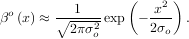
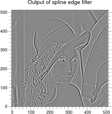
A function to compute this Gaussian for arbitrary x and o is also available (signal.gauss_spline). The following code and Figure uses spline-filtering to compute an edge-image (the second-derivative of a smoothed spline) of Lena’s face which is an array returned by the command lena(). The command signal.sepfir2d was used to apply a separable two-dimensional FIR filter with mirror-symmetric boundary conditions to the spline coefficients. This function is ideally suited for reconstructing samples from spline coefficients and is faster than signal.convolve2d which convolves arbitrary two-dimensional filters and allows for choosing mirror-symmetric boundary conditions.
Filtering is a generic name for any system that modifies an input signal in some way. In SciPy a signal can be thought of as a Numeric array. There are different kinds of filters for different kinds of operations. There are two broad kinds of filtering operations: linear and non-linear. Linear filters can always be reduced to multiplication of the flattened Numeric array by an appropriate matrix resulting in another flattened Numeric array. Of course, this is not usually the best way to compute the filter as the matrices and vectors involved may be huge. For example filtering a 512 × 512 image with this method would require multiplication of a 5122x5122matrix with a 5122 vector. Just trying to store the 5122 × 5122 matrix using a standard Numeric array would require 68,719,476,736 elements. At 4 bytes per element this would require 256GB of memory. In most applications most of the elements of this matrix are zero and a different method for computing the output of the filter is employed.
Many linear filters also have the property of shift-invariance. This means that the filtering operation is the same at different locations in the signal and it implies that the filtering matrix can be constructed from knowledge of one row (or column) of the matrix alone. In this case, the matrix multiplication can be accomplished using Fourier transforms.
Let x![[n]](tutorial83x.png) define a one-dimensional signal indexed by the integer n. Full convolution of two one-dimensional
signals can be expressed as
define a one-dimensional signal indexed by the integer n. Full convolution of two one-dimensional
signals can be expressed as
![∑∞
y[n] = x [k]h[n - k].
k=-∞](tutorial84x.png)
This equation can only be implemented directly if we limit the sequences to finite support sequences that can be
stored in a computer, choose n = 0 to be the starting point of both sequences, let K + 1 be that value for which
y![[n]](tutorial85x.png) = 0 for all n > K + 1 and M + 1 be that value for which x
= 0 for all n > K + 1 and M + 1 be that value for which x![[n]](tutorial86x.png) = 0 for all n > M + 1, then the discrete
convolution expression is
= 0 for all n > M + 1, then the discrete
convolution expression is
![min∑(n,K)
y[n] = x [k]h [n - k].
k=max(n- M,0)](tutorial87x.png)
For convenience assume K ≥ M. Then, more explicitly the output of this operation is
![y[0] = x[0]h [0]
y[1] = x[0]h [1]+ x [1]h[0]
y[2] = x[0]h [2]+ x [1]h[1]+ x[2]h [0]
. . .
.. .. ..
y[M ] = x[0]h [M ]+ x [1]h[M - 1]+ ⋅⋅⋅+ x[M ]h [0]
y[M + 1] = x[1]h [M ]+ x [2]h[M - 1]+ ⋅⋅⋅+ x[M + 1]h[0]
... ... ...
y [K] = x[K - M ]h[M ]+ ⋅⋅⋅+ x[K]h [0]
y[K + 1] = x[K + 1- M ]h[M ]+ ⋅⋅⋅+ x [K] h[1]
.. .. ..
. . .
y[K +M - 1] = x[K - 1]h [M ]+ x [K] h[M - 1]
y[K + M ] = x[K]h [M ].](tutorial88x.png)
 +
+  - 1.
- 1.
One dimensional convolution is implemented in SciPy with the function signal.convolve. This function takes
as inputs the signals x, h, and an optional flag and returns the signal y. The optional flag allows for specification of
which part of the output signal to return. The default value of ’full’ returns the entire signal. If the flag
has a value of ’same’ then only the middle K values are returned starting at y![[⌊M--21⌋]](tutorial91x.png) so that the
output has the same length as the largest input. If the flag has a value of ’valid’ then only the middle
K - M + 1 =
so that the
output has the same length as the largest input. If the flag has a value of ’valid’ then only the middle
K - M + 1 =  -
- + 1 output values are returned where z depends on all of the values of
the smallest input from h
+ 1 output values are returned where z depends on all of the values of
the smallest input from h![[0]](tutorial94x.png) to h
to h![[M ]](tutorial95x.png) . In other words only the values y
. In other words only the values y![[M ]](tutorial96x.png) to y
to y![[K]](tutorial97x.png) inclusive are
returned.
inclusive are
returned.
This same function signal.convolve can actually take N-dimensional arrays as inputs and will return the N-dimensional convolution of the two arrays. The same input flags are available for that case as well.
Correlation is very similar to convolution except for the minus sign becomes a plus sign. Thus
![∞∑
w [n] = y[k]x[n+ k]
k=-∞](tutorial98x.png)
is the (cross) correlation of the signals y and x. For finite-length signals with y![[n]](tutorial99x.png) = 0 outside of the range
= 0 outside of the range ![[0,K]](tutorial100x.png) and x
and x![[n]](tutorial101x.png) = 0 outside of the range
= 0 outside of the range ![[0,M ]](tutorial102x.png) , the summation can simplify to
, the summation can simplify to
![min(K∑,M -n)
w[n] = y[k]x[n + k].
k=max(0,-n)](tutorial103x.png)
Assuming again that K ≥ M this is
![w [- K] = y[K] x[0]
w[- K + 1] = y[K - 1]x[0]+ y[K] x[1]
.. .. ..
. . .
w [M - K] = y[K - M ]x[0]+ y[K - M + 1]x[1]+ ⋅⋅⋅+ y[K] x[M ]
w[M - K + 1] = y[K - M - 1]x [0]+ ⋅⋅⋅+ y[K - 1]x [M ]
. . .
.. .. ..
w[- 1] = y[1]x[0]+ y[2]x [1]+ ⋅⋅⋅+y [M + 1]x [M ]
w [0] = y[0]x[0]+ y[1]x [1]+ ⋅⋅⋅+y [M ]x [M ]
w [1] = y[0]x[1]+ y[1]x [2]+ ⋅⋅⋅+y [M - 1]x [M ]
w [2] = y[0]x[2]+ y[1]x [3]+ ⋅⋅⋅+y [M - 2]x [M ]
.. .. ..
. . .
w[M - 1] = y[0]x[M - 1]+ y[1]x[M ]
w [M ] = y[0]x[M ].](tutorial104x.png)
The SciPy function signal.correlate implements this operation. Equivalent flags are available for this
operation to return the full K + M + 1 length sequence (’full’) or a sequence with the same size as the largest
sequence starting at w![[- K + ⌊M--1⌋]
2](tutorial105x.png) (’same’) or a sequence where the values depend on all the values of
the smallest sequence (’valid’). This final option returns the K - M + 1 values w
(’same’) or a sequence where the values depend on all the values of
the smallest sequence (’valid’). This final option returns the K - M + 1 values w![[M - K]](tutorial106x.png) to w
to w![[0]](tutorial107x.png) inclusive.
inclusive.
The function signal.correlate can also take arbitrary N-dimensional arrays as input and return the N-dimensional convolution of the two arrays on output.
When N = 2, signal.correlate and/or signal.convolve can be used to construct arbitrary image filters to perform actions such as blurring, enhancing, and edge-detection for an image.
Convolution is mainly used for filtering when one of the signals is much smaller than the other (K ≫ M), otherwise linear filtering is more easily accomplished in the frequency domain (see Fourier Transforms).
A general class of linear one-dimensional filters (that includes convolution filters) are filters described by the difference equation
![∑N M∑
aky [n - k] = bkx[n- k]
k=0 k=0](tutorial108x.png)
where x![[n]](tutorial109x.png) is the input sequence and y
is the input sequence and y![[n]](tutorial110x.png) is the output sequence. If we assume initial rest so that y
is the output sequence. If we assume initial rest so that y![[n]](tutorial111x.png) = 0 for
n < 0, then this kind of filter can be implemented using convolution. However, the convolution filter
sequence h
= 0 for
n < 0, then this kind of filter can be implemented using convolution. However, the convolution filter
sequence h![[n]](tutorial112x.png) could be infinite if ak
could be infinite if ak 0 for k ≥ 1. In addition, this general class of linear filter allows
initial conditions to be placed on y
0 for k ≥ 1. In addition, this general class of linear filter allows
initial conditions to be placed on y![[n]](tutorial114x.png) for n < 0 resulting in a filter that cannot be expressed using
convolution.
for n < 0 resulting in a filter that cannot be expressed using
convolution.
The difference equation filter can be thought of as finding y![[n]](tutorial115x.png) recursively in terms of it’s previous
values
recursively in terms of it’s previous
values
![a0y[n] = - a1y[n - 1]- ⋅⋅⋅- aNy [n - N]+ ⋅⋅⋅+ b0x [n]+ ⋅⋅⋅+ bMx [n - M ].](tutorial116x.png)
Often a0 = 1 is chosen for normalization. The implementation in SciPy of this general difference equation filter is a little more complicated then would be implied by the previous equation. It is implemented so that only one signal needs to be delayed. The actual implementation equations are (assuming a0 = 1).
![y [n] = b x[n]+ z [n - 1]
0 0
z0 [n] = b1x[n]+ z1[n - 1]- a1y [n]
z1 [n] = b2x[n]+ z2[n - 1]- a2y [n]
.. .. ..
. . .
zK-2 [n] = bK- 1x [n]+ zK -1[n - 1]- aK-1y[n]
zK-1 [n] = bKx [n]- aKy [n],](tutorial117x.png)
 . Note that bK = 0 if K > M and aK = 0 if K > N. In this way, the output at
time n depends only on the input at time n and the value of z0 at the previous time. This can always
be calculated as long as the K values z0
. Note that bK = 0 if K > M and aK = 0 if K > N. In this way, the output at
time n depends only on the input at time n and the value of z0 at the previous time. This can always
be calculated as long as the K values z0![[n - 1]](tutorial119x.png) …zK-1
…zK-1![[n- 1]](tutorial120x.png) are computed and stored at each time
step.
are computed and stored at each time
step.
The difference-equation filter is called using the command signal.lfilter in SciPy. This command takes as inputs
the vector b, the vector, a, a signal x and returns the vector y (the same length as x) computed using the equation
given above. If x is N-dimensional, then the filter is computed along the axis provided. If, desired, initial
conditions providing the values of z0![[- 1]](tutorial121x.png) to zK-1
to zK-1![[- 1]](tutorial122x.png) can be provided or else it will be assumed
that they are all zero. If initial conditions are provided, then the final conditions on the intermediate
variables are also returned. These could be used, for example, to restart the calculation in the same
state.
can be provided or else it will be assumed
that they are all zero. If initial conditions are provided, then the final conditions on the intermediate
variables are also returned. These could be used, for example, to restart the calculation in the same
state.
Sometimes it is more convenient to express the initial conditions in terms of the signals x![[n]](tutorial123x.png) and y
and y![[n]](tutorial124x.png) . In other
words, perhaps you have the values of x
. In other
words, perhaps you have the values of x![[- M ]](tutorial125x.png) to x
to x![[- 1]](tutorial126x.png) and the values of y
and the values of y![[- N ]](tutorial127x.png) to y
to y![[- 1]](tutorial128x.png) and would like to
determine what values of zm
and would like to
determine what values of zm![[- 1]](tutorial129x.png) should be delivered as initial conditions to the difference-equation filter. It is not
difficult to show that for 0 ≤ m < K,
should be delivered as initial conditions to the difference-equation filter. It is not
difficult to show that for 0 ≤ m < K,
![K-∑m -1
zm [n] = (bm+p+1x [n- p]- am+p+1y [n - p]).
p=0](tutorial130x.png)
Using this formula we can find the intial condition vector z0![[- 1]](tutorial131x.png) to zK-1
to zK-1![[- 1]](tutorial132x.png) given initial conditions on y (and x).
The command signal.lfiltic performs this function.
given initial conditions on y (and x).
The command signal.lfiltic performs this function.
The signal processing package affords many more filters as well.
Median Filter A median filter is commonly applied when noise is markedly non-Gaussian or when it is desired to preserve edges. The median filter works by sorting all of the array pixel values in a rectangular region surrounding the point of interest. The sample median of this list of neighborhood pixel values is used as the value for the output array. The sample median is the middle array value in a sorted list of neighborhood values. If there are an even number of elements in the neighborhood, then the average of the middle two values is used as the median. A general purpose median filter that works on N-dimensional arrays is signal.medfilt. A specialized version that works only for two-dimensional arrays is available as signal.medfilt2d.
Order Filter A median filter is a specific example of a more general class of filters called order filters. To compute the output at a particular pixel, all order filters use the array values in a region surrounding that pixel. These array values are sorted and then one of them is selected as the output value. For the median filter, the sample median of the list of array values is used as the output. A general order filter allows the user to select which of the sorted values will be used as the output. So, for example one could choose to pick the maximum in the list or the minimum. The order filter takes an additional argument besides the input array and the region mask that specifies which of the elements in the sorted list of neighbor array values should be used as the output. The command to perform an order filter is signal.order_filter.
Wiener filter The Wiener filter is a simple deblurring filter for denoising images. This is not the Wiener filter commonly described in image reconstruction problems but instead it is a simple, local-mean filter. Let x be the input signal, then the output is

Where mx is the local estimate of the mean and σx2 is the local estimate of the variance. The window for these estimates is an optional input parameter (default is 3 × 3). The parameter σ2 is a threshold noise parameter. If σ is not given then it is estimated as the average of the local variances.
Hilbert filter
The Hilbert transform constructs the complex-valued analytic signal from a real signal. For example if
x = cosωn then y = hilbert would return (except near the edges) y = exp
 . In the frequency domain, the
hilbert transform performs
. In the frequency domain, the
hilbert transform performs

where H is 2 for positive frequencies, 0 for negative frequencies and 1 for zero-frequencies.
When SciPy is built using the optimized ATLAS LAPACK and BLAS libraries, it has very fast linear algebra capabilities. If you dig deep enough, all of the raw lapack and blas libraries are available for your use for even more speed. In this section, some easier-to-use interfaces to these routines are described.
All of these linear algebra routines expect an object that can be converted into a 2-dimensional array. The output of these routines is also a two-dimensional array. There is a matrix class defined in Numeric that scipy inherits and extends. You can initialize this class with an appropriate Numeric array in order to get objects for which multiplication is matrix-multiplication instead of the default, element-by-element multiplication.
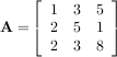
The matrix class is initialized with the SciPy command mat which is just convenient short-hand for Matrix.Matrix. If you are going to be doing a lot of matrix-math, it is convenient to convert arrays into matrices using this command. One convencience of using the mat command is that you can enter two-dimensional matrices in using MATLAB-like syntax with commas or spaces separating columns and semicolons separting rows as long as the matrix is placed in a string passed to mat.
The inverse of a matrix A is the matrix B such that AB = I where I is the identity matrix consisting of ones down the main diagonal. Usually B is denoted B = A-1. In SciPy, the matrix inverse of the Numeric array, A, is obtained using linalg.inv(A), or using A.I if A is a Matrix. For example, let
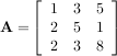
then

The following example demonstrates this computation in SciPy
Solving linear systems of equations is straightforward using the scipy command linalg.solve. This command expects an input matrix and a right-hand-side vector. The solution vector is then computed. An option for entering a symmetrix matrix is offered which can speed up the processing when applicable. As an example, suppose it is desired to solve the following simultaneous equations:


However, it is better to use the linalg.solve command which can be faster and more numerically stable. In this case it gives the same answer as shown in the following example:
The determinant of a square matrix A is often denoted  and is a quantity often used in linear algebra. Suppose
aij are the elements of the matrix A and let Mij =
and is a quantity often used in linear algebra. Suppose
aij are the elements of the matrix A and let Mij =  be the determinant of the matrix left by removing the ith
row and jthcolumn from A. Then for any row i,
be the determinant of the matrix left by removing the ith
row and jthcolumn from A. Then for any row i,

This is a recursive way to define the determinant where the base case is defined by accepting that the determinant of a 1 × 1 matrix is the only matrix element. In SciPy the determinant can be calculated with linalg.det. For example, the determinant of
is

Matrix and vector norms can also be computed with SciPy. A wide range of norm definitions are available using different parameters to the order argument of linalg.norm. This function takes a rank-1 (vectors) or a rank-2 (matrices) array and an optional order argument (default is 2). Based on these inputs a vector or matrix norm of the requested order is computed.
For vector x, the order parameter can be any real number including inf or -inf. The computed norm is

For matrix A the only valid values for norm are ±2,±1, ±inf, and ’fro’ (or ’f’) Thus,

where σi are the singular values of A.
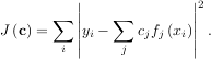
Linear least-squares problems occur in many branches of applied mathematics. In this problem a set of linear scaling
coefficients is sought that allow a model to fit data. In particular it is assumed that data yi is related to data xi
through a set of coefficients cj and model functions fj via the model

where εi represents uncertainty in the data. The strategy of least squares is to pick the coefficients cj to minimize
Theoretically, a global minimum will occur when
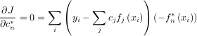
or
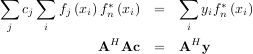

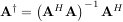
When AHA is invertible, then
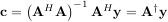
where A† is called the pseudo-inverse of A. Notice that using this definition of A the model can be written

The command linalg.lstsq will solve the linear least squares problem for c given A and y. In addition linalg.pinv or linalg.pinv2 (uses a different method based on singular value decomposition) will find A† given A.
The following example and figure demonstrate the use of linalg.lstsq and linalg.pinv for solving a data-fitting problem. The data shown below were generated using the model:

where xi = 0.1i for i = 1…10, c1 = 5, and c2 = 4. Noise is added to yi and the coefficients c1 and c2 are estimated using linear least squares.
c1,c2= 5.0,2.0
i = r_[1:11] xi = 0.1*i yi = c1*exp(-xi)+c2*xi zi = yi + 0.05*max(yi)*randn(len(yi)) A = c_[exp(-xi)[:,NewAxis],xi[:,NewAxis]] c,resid,rank,sigma = linalg.lstsq(A,zi) xi2 = r_[0.1:1.0:100j] yi2 = c[0]*exp(-xi2) + c[1]*xi2 xplt.plot(xi,zi,’x’,xi2,yi2) xplt.limits(0,1.1,3.0,5.5) xplt.xlabel(’x_i’) xplt.title(’Data fitting with linalg.lstsq’) xplt.eps(’lstsq_fit’) |
 |
The generalized inverse is calculated using the command linalg.pinv or linalg.pinv2. These two commands differ in how they compute the generalized inverse. The first uses the linalg.lstsq algorithm while the second uses singular value decomposition. Let A be an M × N matrix, then if M > N the generalized inverse is
while if M < N matrix the generalized inverse is

In both cases for M = N, then

as long as A is invertible.
In many applications it is useful to decompose a matrix using other representations. There are several decompositions supported SciPy.
The eigenvalue-eigenvector problem is one of the most commonly employed linear algebra operations. In one popular form, the eigenvalue-eigenvector problem is to find for some square matrix A scalars λ and corresponding vectors v such that

For an N × N matrix, there are N (not necessarily distinct) eigenvalues — roots of the (characteristic) polynomial

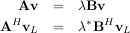
The eigenvectors, v, are also sometimes called right eigenvectors to distinguish them from another set of left eigenvectors that satisfy

or

With it’s default optional arguments, the command linalg.eig returns λ and v. However, it can also return vL and just λ by itself (linalg.eigvals returns just λ as well).
In addtion, linalg.eig can also solve the more general eigenvalue problem

where V is the collection of eigenvectors into columns and Λ is a diagonal matrix of eigenvalues.
By definition, eigenvectors are only defined up to a constant scale factor. In SciPy, the scaling factor for the
eigenvectors is chosen so that  2 = ∑
ivi2 = 1.
2 = ∑
ivi2 = 1.
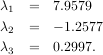
As an example, consider finding the eigenvalues and eigenvectors of the matrix
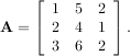
The characteristic polynomial is
![∣A - λI∣ = (1- λ)[(4- λ)(2- λ)- 6]-
5[2(2- λ)- 3]+ 2[12- 3(4 - λ)]
= - λ3 + 7λ2 + 8λ - 3.](tutorial169x.png)
Singular Value Decompostion (SVD) can be thought of as an extension of the eigenvalue problem to matrices that
are not square. Let A be an M ×N matrix with M and N arbitrary. The matrices AHA and AAH are square hermitian
matrices3
of size N × N and M × M respectively. It is known that the eigenvalues of square hermitian
matrices are real and non-negative. In addtion, there are at most min identical non-zero
eigenvalues of AHA and AAH. Define these positive eigenvalues as σi2. The square-root of these
are called singular values of A. The eigenvectors of AHA are collected by columns into an N × N
unitary4
matrix V while the eigenvectors of AAH are collected by columns in the unitary matrix U, the singular
values are collected in an M × N zero matrix Σ with main diagonal entries set to the singular values.
Then
identical non-zero
eigenvalues of AHA and AAH. Define these positive eigenvalues as σi2. The square-root of these
are called singular values of A. The eigenvectors of AHA are collected by columns into an N × N
unitary4
matrix V while the eigenvectors of AAH are collected by columns in the unitary matrix U, the singular
values are collected in an M × N zero matrix Σ with main diagonal entries set to the singular values.
Then

is the singular-value decomposition of A. Every matrix has a singular value decomposition. Sometimes, the singular values are called the spectrum of A. The command linalg.svd will return U, VH, and σi as an array of the singular values. To obtain the matrix Σ use linalg.diagsvd. The following example illustrates the use of linalg.svd.
The LU decompostion finds a representation for the M × N matrix A as

where P is an M ×M permutation matrix (a permutation of the rows of the identity matrix), L is in M ×K lower
triangular or trapezoidal matrix (K = min ) with unit-diagonal, and U is an upper triangular or trapezoidal
matrix. The SciPy command for this decomposition is linalg.lu.
) with unit-diagonal, and U is an upper triangular or trapezoidal
matrix. The SciPy command for this decomposition is linalg.lu.
Such a decomposition is often useful for solving many simultaneous equations where the left-hand-side does not change but the right hand side does. For example, suppose we are going to solve

for many different bi. The LU decomposition allows this to be written as

Because L is lower-triangular, the equation can be solved for Uxi and finally xi very rapidly using forward- and back-substitution. An initial time spent factoring A allows for very rapid solution of similar systems of equations in the future. If the intent for performing LU decomposition is for solving linear systems then the command linalg.lu_factor should be used followed by repeated applications of the command linalg.lu_solve to solve the system for each new right-hand-side.
Cholesky decomposition is a special case of LU decomposition applicable to Hermitian positive definite matrices. When A = AH and xHAx ≥ 0 for all x, then decompositions of A can be found so that

The QR decomposition (sometimes called a polar decomposition) works for any M ×N array and finds an M ×M unitary matrix Q and an M × N upper-trapezoidal matrix R such that

Notice that if the SVD of A is known then the QR decomposition can be found
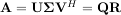
implies that Q = U and R = ΣVH. Note, however, that in SciPy independent algorithms are used to find QR and SVD decompositions. The command for QR decomposition is linalg.qr.
For a square N × N matrix, A, the Schur decomposition finds (not-necessarily unique) matrices T and Z such that

where Z is a unitary matrix and T is either upper-triangular or quasi-upper triangular depending on whether or not a real schur form or complex schur form is requested. For a real schur form both T and Z are real-valued when A is real-valued. When A is a real-valued matrix the real schur form is only quasi-upper triangular because 2 × 2 blocks extrude from the main diagonal corresponding to any complex-valued eigenvalues. The command linalg.schur finds the Schur decomposition while the command linalg.rsf2csf converts T and Z from a real Schur form to a complex Schur form. The Schur form is especially useful in calculating functions of matrices.
The following example illustrates the schur decomposition:
Consider the function f with Taylor series expansion

A matrix function can be defined using this Taylor series for the square matrix A as

While, this serves as a useful representation of a matrix function, it is rarely the best way to calculate a matrix function.
The matrix exponential is one of the more common matrix functions. It can be defined for square matrices as

The command linalg.expm3 uses this Taylor series definition to compute the matrix exponential. Due to poor convergence properties it is not often used.
Another method to compute the matrix exponential is to find an eigenvalue decomposition of A:

and note that

where the matrix exponential of the diagonal matrix Λ is just the exponential of its elements. This method is implemented in linalg.expm2.
The preferred method for implementing the matrix exponential is to use scaling and a Padé approximation for ex. This algorithm is implemented as linalg.expm.
The inverse of the matrix exponential is the matrix logarithm defined as the inverse of the matrix exponential.

The matrix logarithm can be obtained with linalg.logm.
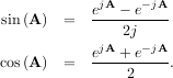
The trigonometric functions sin, cos, and tan are implemented for matrices in linalg.sinm, linalg.cosm, and linalg.tanm respectively. The matrix sin and cosine can be defined using Euler’s identity as
![tan(x) = sin(x)-= [cos(x)]-1 sin(x)
cos(x)](tutorial189x.png)
and so the matrix tangent is defined as
![[cos(A)]-1sin (A) .](tutorial190x.png)
The hyperbolic trigonemetric functions sinh, cosh, and tanh can also be defined for matrices using the familiar definitions:
![eA---e--A-
sinh(A) = 2
eA-+-e--A-
cosh(A) = 2
tanh(A) = [cosh(A)]-1sinh (A).](tutorial191x.png)
Finally, any arbitrary function that takes one complex number and returns a complex number can be called as a matrix function using the command linalg.funm. This command takes the matrix and an arbitrary Python function. It then implements an algorithm from Golub and Van Loan’s book “Matrix Computations” to compute function applied to the matrix using a Schur decomposition. Note that the function needs to accept complex numbers as input in order to work with this algorithm. For example the following code computes the zeroth-order Bessel function applied to a matrix.
SciPy has a tremendous number of basic statistics routines with more easily added by the end user (if you create one please contribute it). All of the statistics functions are located in the sub-package stats and a fairly complete listing of these functions can be had using info(stats).
There are two general distribution classes that have been implemented for encapsulating continuous random variables and discrete random variables. Over 80 continuous random variables and 10 discrete random variables have been implemented using these classes. The list of the random variables available is in the docstring for the stats sub-package. A detailed description of each of them is also located in the files continuous.lyx and discrete.lyx in the stats sub-directories.
If you have the Python Imaging Library installed, SciPy provides some convenient functions that make use of it’s facilities particularly for reading, writing, displaying, and rotating images. In SciPy an image is always a two- or three-dimensional array. Gray-scale, and colormap images are always two-dimensional arrays while RGB images are three-dimensional with the third dimension specifying the channel.
Commands available include
The underlying graphics library for xplt is the pygist library. All of the commands of pygist are available under xplt as well. For more information on the pygist commands you can read the documentation of that package in html here http://bonsai.ims.u-tokyo.ac.jp/~mdehoon/software/python/pygist_html/pygist.html or in pdf at this location http://bonsai.ims.u-tokyo.ac.jp/~mdehoon/software/python/pygist.pdf. It should be noted that xplt is available on Unix and Windows and should work on MacOS X.